Review
. 2016 May 24:5:F1000 Faculty Rev-992.
doi: 10.12688/f1000research.7698.1. eCollection 2016.

Dynamical systems, attractors, and neural circuits

Affiliations
Review

Dynamical systems, attractors, and neural circuits

Paul Miller. F1000Res. .

Abstract

Biology is the study of dynamical systems. Yet most of us working in biology have limited pedagogical training in the theory of dynamical systems, an unfortunate historical fact that can be remedied for future generations of life scientists. In my particular field of systems neuroscience, neural circuits are rife with nonlinearities at all levels of description, rendering simple methodologies and our own intuition unreliable. Therefore, our ideas are likely to be wrong unless informed by good models. These models should be based on the mathematical theories of dynamical systems since functioning neurons are dynamic-they change their membrane potential and firing rates with time. Thus, selecting the appropriate type of dynamical system upon which to base a model is an important first step in the modeling process. This step all too easily goes awry, in part because there are many frameworks to choose from, in part because the sparsely sampled data can be consistent with a variety of dynamical processes, and in part because each modeler has a preferred modeling approach that is difficult to move away from. This brief review summarizes some of the main dynamical paradigms that can arise in neural circuits, with comments on what they can achieve computationally and what signatures might reveal their presence within empirical data. I provide examples of different dynamical systems using simple circuits of two or three cells, emphasizing that any one connectivity pattern is compatible with multiple, diverse functions.

Keywords: Heteroclinics; Marginal states; Oscillating systems; Point attractors; continuous attractors; cyclic attractors; hidden Markov model; limit cycles; line attractors; strange attractors.


Conflict of interest statement

Competing interests: The author declares that he has no competing interests.

No competing interests were disclosed.

Figures
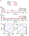
Figure 1.
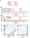
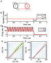
Figure 1.. A single point attractor is present without input and a different one with input in a threshold-linear two-unit circuit.
( A) Diagram of the model circuit. Arrows indicate excitatory connections, and balls indicate inhibitory connections between units. ( B) Applied current as a function of time. Two different sized pulses of current are applied to unit 1. ( C) Firing rate as a function of time in the coupled network. During each current step, a new attractor is produced, but following current offset the original activity state is reached. ( D) Any particular combination of the firing rates of the two units (x-axis is rate of unit 1, y-axis is rate of unit 2) determines the way those firing rates change in time (arrows). Starting from any pair of firing rates, any trajectory following arrows terminates at the point of intersection of the two lines. Red line: nullcline for unit 2—the value of r(2) at which dr(2)/dt = 0 (its fixed point) given a value of r(1). Since unit 1 excites unit 2, the fixed point for r(2) increases with r(1). Black line: nullcline for unit 1—the value of r(1) at which dr(1)/dt = 0 (its fixed point) given a value of r(2). Since unit 2 inhibits neuron 1, the fixed point for r(1) decreases with r(2). The crossing point of the nullclines is a fixed point of the whole system. The fixed point is stable (so is an attractor state) because arrows converge on the fixed point. ( E) As in (D) but the solution during the second pulse of applied current. The applied current shifts the nullcline for r(1) so that the fixed point of the system is at much higher values of r(1) and r(2). For parameters, see supporting Matlab code, “dynamics_two_units.m”.
Figure 2.
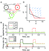
Figure 2.. A multistable attractor network can be switched between states to encode distinct memories through persistent activity in a threshold-linear two-unit circuit.
( A) Diagram of the model circuit. Arrows indicate excitatory connections, and balls indicate inhibitory connections. The strong self-excitatory feedback renders each unit unstable once active. ( B) Applied current as a function of time. The first pulse is applied to unit 1, the second to unit 2. ( C) Firing rate as a function of time in the coupled network reveals three different activity states: both units inactive or either one active. The activity persists after offset of the applied current—a signature of multistability—so retains memory of past inputs. ( D) Any particular combination of the firing rates of the two neurons (x-axis is rate of neuron 1, y-axis is rate of neuron 2) determines the way those firing rates change in time (arrows). Depending on the initial pair of firing rates, a trajectory following arrows terminates at one of the points of intersection of the two lines, either (0,0) or (100,0) or (0,100). The intersections at the midpoints of the lines are unstable—if activity of unit 1 is under 50 Hz, it decays to 0; if it is over 50 Hz, it will increase to 100 Hz (if unit 2 is inactive). Red line: nullcline for neuron 2—the value of r(2) at which dr(2)/dt = 0 (its fixed point) given a value of r(1). Since neuron 1 excites neuron 2, the fixed point for r(2) increases with r(1). Black line: nullcline for neuron 1—the value of r(1) at which dr(1)/dt = 0 (its fixed point) given a value of r(2). Since neuron 2 inhibits neuron 1, the fixed point for r(1) decreases with r(2). The crossing point of the nullclines is a fixed point of the whole system. The fixed point is stable (so is an attractor state) because arrows converge on the fixed point. ( E) As in ( D) but the solution during the second pulse of applied current. The applied current shifts the nullcline for r(1) so that the only fixed point of the system is at (100,0). For parameters, see supporting Matlab code, “dynamics_two_units.m”.
Figure 3.
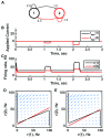
Figure 3.. The “paradoxical” shift of a single point attractor in the inhibition-stabilized regime in a threshold-linear two-unit circuit.
( A) Diagram of the model circuit. Arrows indicate excitatory connections, and balls indicate inhibitory connections between units. Architecture is identical to that in Figure 1. ( B) Applied current as a function of time. Two different sized inhibitory pulses of current are applied to unit 2. ( C) Firing rate as a function of time in the coupled network. During each current step, a new attractor is produced, but following current offset the original activity state is reached. When inhibition is applied to unit 2, the rates of both unit 1 and unit 2 increase as a result of the ensuing net within-circuit increase in excitation to both units. The “paradox” lies in that external inhibition to unit 2 results in an increase in its rate (due to internal raised excitation) and, even more counter-intuitively, unit 1 stabilizes at a higher firing rate in the presence of greater inhibitory input from unit 2. ( D) Any particular combination of the firing rates of the two units (x-axis is rate of unit 1, y-axis is rate of unit 2) determines the way those firing rates change in time (arrows). Starting from any pair of firing rates, any trajectory following arrows terminates at the point of intersection of the two lines. Red line: nullcline for unit 2—the value of r(2) at which dr(2)/dt = 0 (its fixed point) given a value of r(1). Since unit 1 excites unit 2, the fixed point for r(2) increases with r(1). Black line: nullcline for unit 1—the value of r(1) at which dr(1)/dt = 0 (its fixed point) given a value of r(2). Since unit 2 inhibits unit 1, at high enough r(2) only r(1) = 0 is possible and at low r(2) only r(1) = 100 is possible. The line joining the minimum and maximum values of r(1) would normally be of unstable fixed points, but in this system it is stabilized. The crossing point of the nullclines is the fixed point of the whole system. The fixed point is stable (so is an attractor state) because arrows converge on the fixed point. ( E) As in ( D) but the solution during the second pulse of applied current. The inhibitory applied current shifts the nullcline for r(2) down, and the result is that the fixed point of the system moves to higher values of both r(1) and r(2). For parameters, see supporting Matlab code, “dynamics_two_units.m”.
Figure 4.
Figure 4.. Bistability with low stable firing rates in the inhibition-stabilized threshold-linear three-unit circuit.
( A) Diagram of the model circuit. Arrows indicate excitatory connections, and balls indicate inhibitory connections between units. A third unit is added to the architecture of Figure 3. ( B) Applied current as a function of time. The first current pulse is applied to unit 1, and the second is applied to unit 3. A small amount of noise is added to the current to prevent the system resting at an unstable symmetric state, toward which it is otherwise drawn. ( C) Firing rate as a function of time in the coupled network. The current steps switch activity between stable states in which no neuron’s activity is greater than 10 Hz—note the difference in rates from the “traditional” bistability of Figure 2. ( D) Any particular combination of the firing rates of the three units (x-axis is rate of unit 1, y-axis is rate of unit 3) determines the way those firing rates change in time (arrows). Only a plane out of the full three-dimensional space of arrows is shown—the plane corresponding to dr(3)/dt = 0. Starting from any pair of firing rates, any trajectory following arrows terminates at the point of intersection of the two lines. Red line: nullcline for unit 2—the value of r(2) at which dr(2)/dt = 0 (its fixed point) given a value of r(1). Black line: nullcline for unit 1—the value of r(1) at which dr(1)/dt = 0 (its fixed point) given a value of r(2). Since unit 2 inhibits neuron 1, the fixed point for r(1) decreases with r(2). The crossing points of the nullclines are fixed points of the whole system. The asymmetric fixed points are stable (so are attractor states) because arrows converge on them, whereas the intervening symmetric fixed point is unstable. For parameters, see supporting Matlab code, “dynamics_three_units.m”.
Figure 5.
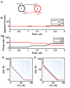
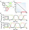
Figure 5.. A marginal state or continuous/line attractor is produced by careful tuning of the connection strengths in a threshold-linear two-unit circuit.
( A) Diagram of the model circuit. Arrows indicate excitatory connections, and balls indicate inhibitory connections between units. The architecture is identical to that of Figure 2. ( B) Applied current as a function of time. Two very small pulses of current are applied to unit 1. ( C) Firing rate as a function of time in the coupled network. During each current step, the firing rate of unit 1 increases linearly because of the applied current. Inhibitory feedback to unit 2 causes a linear decrease in its firing rate. Upon stimulus offset, the firing rate reached is maintained. ( D) Any particular combination of the firing rates of the two units (x-axis is rate of unit 1, y-axis is rate of unit 2) determines the way those firing rates change in time (arrows). Starting from any pair of firing rates, any trajectory following arrows terminates at a point where the two lines overlap each other. Red line: nullcline for unit 2—the value of r(2) at which dr(2)/dt = 0 (its fixed point) given a value of r(1). Black line: nullcline for unit 1—the value of r(1) at which dr(1)/dt = 0 (its fixed point) given a value of r(2). Since the two units inhibit each other, the overlapping lines have negative gradient. ( E) A small applied current to unit 1 shifts its nullcline to the right slightly. Now the only fixed point is where the two lines intersect at r(2) = 0, but in the region between the two parallel nullclines, the rate of change is small (note the small arrows parallel to the lines) so firing rates change gradually. For parameters, see supporting Matlab code, “dynamics_two_units.m”.
Figure 6.
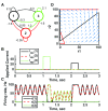
Figure 6.. An oscillator produced by directed excitatory and inhibitory connections in a bistable threshold-linear two-unit circuit.
( A) Diagram of the model circuit. Arrows indicate excitatory connections, and balls indicate inhibitory connections between units. The architecture is identical to that of Figure 1 and Figure 3. ( B) Applied current as a function of time. An inhibitory pulse of current is applied to unit 1. ( C) Firing rate as a function of time in the coupled network. Oscillations are switched off by the inhibition to unit 1, so the system has two stable attractors: one a limit cycle, the other a point attractor. ( D) Any particular combination of the firing rates of the two units (x-axis is rate of unit 1, y-axis is rate of unit 2) determines the way those firing rates change in time (arrows). Depending on the starting point, a trajectory following the arrows will fall on the limit cycle (the green closed orbit, which represents the coordinated variation of firing rate with time during the oscillations) or will reach the fixed point at the origin. Red line: nullcline for unit 2—the value of r(2) at which dr(2)/dt = 0 (its fixed point) given a value of r(1). Since unit 1 excites unit 2, the fixed point for r(2) increases with r(1). Black line: nullcline for unit 1—the value of r(1) at which dr(1)/dt = 0 (its fixed point) given a value of r(2). Crossing points of the nullclines are the fixed points of the whole system, but the one within the limit cycle is unstable, as is the one with r(2) = 0 but r(1) > 0. ( E) As in ( D) but the solution during the inhibitory pulse of applied current. The inhibitory current shifts the nullcline for r(1) down, and the result is that all trajectories terminate at the origin. For parameters, see supporting Matlab code, “dynamics_two_units.m”.
Figure 7.
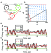
Figure 7.. Switching between two distinct oscillators in a bistable threshold-linear three-unit circuit.
( A) Diagram of the model circuit. Arrows indicate excitatory connections, and balls indicate inhibitory connections between units. Architecture is identical to that of Figure 4. ( B) Applied current as a function of time. The first current pulse is applied to unit 3, and the second is applied to unit 1. ( C) Firing rate as a function of time in the coupled network. The current steps switch activity between two stable states with different frequencies of oscillation. ( D) Any particular combination of the firing rates of the three units (x-axis is rate of unit 1, y-axis is rate of unit 3) determines the way those firing rates change in time (arrows). Only a plane out of the full three-dimensional space of arrows is shown: the plane corresponding to dr(3)/dt = 0. Red line: nullcline for unit 2—the value of r(2) at which dr(2)/dt = 0 (its fixed point) given a value of r(1). Black line: nullcline for unit 1—the value of r(1) at which dr(1)/dt = 0 (its fixed point) given a value of r(2). The crossing points of the nullclines are fixed points of the whole system, none of which is stable in this example. For parameters, see supporting Matlab code, “dynamics_three_units.m”.
Figure 8.
Figure 8.. Chaotic activity in a threshold-linear three-unit circuit.
( A) Diagram of the model circuit. Arrows indicate excitatory connections, and balls indicate inhibitory connections between units. Architecture is identical to that of Figure 4 and Figure 7. ( B, C) Firing rate as a function of time in the coupled network, from two imperceptibly different initial conditions. No applied current is present. The miniscule difference in initial conditions is amplified over time, so, for example, unit 3 produces a small burst of activity after 1.5 s in ( D), but that burst is absent from ( C). ( D) Any particular combination of the firing rates of the three units (x-axis is rate of unit 1, y-axis is rate of unit 3) determines the way those firing rates change in time (arrows). Only a plane out of the full three-dimensional space of arrows is shown: the plane corresponding to dr(2)/dt = 0. Red line: nullcline for unit 2—the value of r(2) at which dr(2)/dt = 0 (its fixed point) given a value of r(1). Black line: nullcline for unit 1—the value of r(1) at which dr(1)/dt = 0 (its fixed point) given a value of r(2). The crossing points of the nullclines are unstable fixed points of the whole system. For parameters, see supporting Matlab code, “dynamics_three_units.m”.
Figure 9.
Figure 9.. Heteroclinic orbits in a threshold-linear three-unit circuit.
( A) Diagram of the model circuit. Arrows indicate excitatory connections, and balls indicate inhibitory connections between units. ( B, C) Firing rate as a function of time in the coupled network from different initial conditions (near the fixed points) with no applied current. Activity is initially slow to move away from the vicinity of the fixed point (along its unstable direction) but after a cycle returns to the vicinity of the same fixed point (along its stable direction). ( D) Any particular combination of the firing rates of the three units (x-axis is rate of unit 1, y-axis is rate of unit 3) determines the way those firing rates change in time (arrows). Only a plane out of the full three-dimensional space of arrows is shown: the plane corresponding to dr(2)/dt = 0. Red line: nullcline for unit 2—the value of r(2) at which dr(2)/dt = 0 (its fixed point) given a value of r(1). Black line: nullcline for unit 1—the value of r(1) at which dr(1)/dt = 0 (its fixed point) given a value of r(2). The crossing points of the nullclines are fixed points of the whole system, in this case at r(1) = 100, r(2) = 0, and r(3) = 0 and at r(1) = 0, r(2) = 100, and r(3) = 100. The fixed points are saddle points in that firing rates can either approach the fixed point or move away from it, depending on the precise set of rates. For parameters, see supporting Matlab code, “dynamics_three_units.m”.

References

    1. Izhikevich EM: Solving the distal reward problem through linkage of STDP and dopamine signaling. Cereb Cortex. 2007;17(10):2443–52. 10.1093/cercor/bhl152 - DOI - PubMed
    1. Strogatz SH: Nonlinear Dynamics and Chaos.Boulder, CO: Westview Press,2015. Reference Source
    1. Dayan P, Abbott LF: Theoretical Neuroscience. MIT Press,2001. Reference Source
    1. Sussillo D, Abbott LF: Generating coherent patterns of activity from chaotic neural networks. Neuron. 2009;63(4):544–57. 10.1016/j.neuron.2009.07.018 - DOI - PMC - PubMed
    1. Rigotti M, Ben Dayan Rubin D, Wang XJ, et al. : Internal representation of task rules by recurrent dynamics: the importance of the diversity of neural responses. Front Comput Neurosci. 2010;4:24. 10.3389/fncom.2010.00024 - DOI - PMC - PubMed

LinkOut - more resources