Understanding the changes of cone reflectance in adaptive optics flood illumination retinal images over three years

Abstract

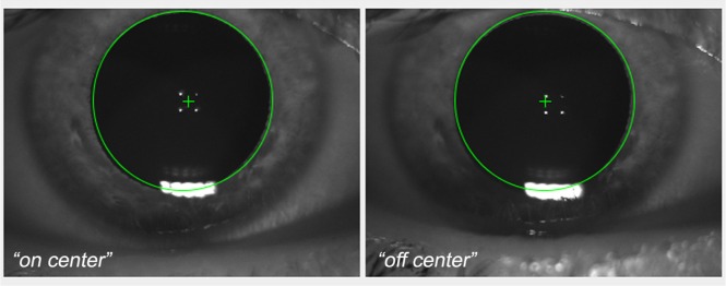
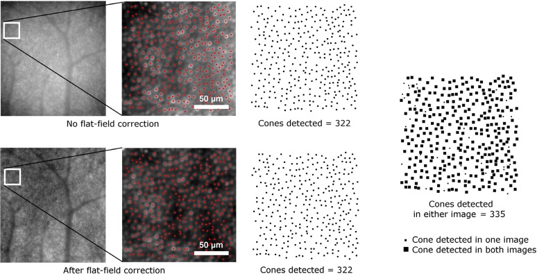
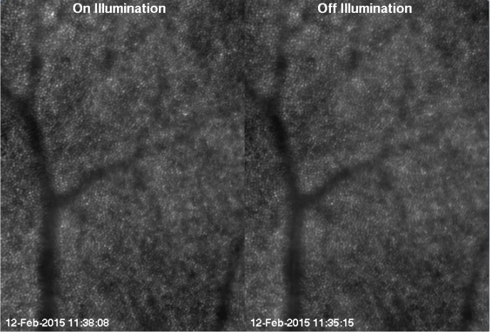
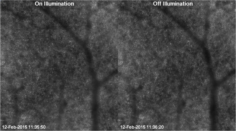
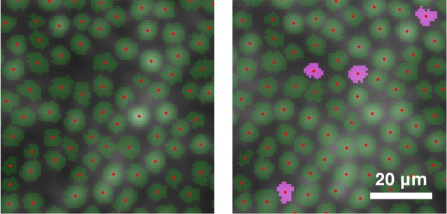
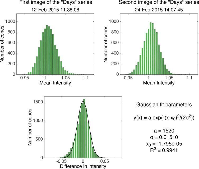
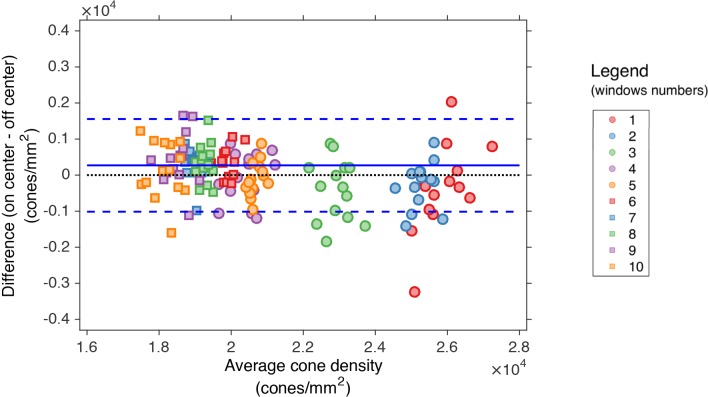
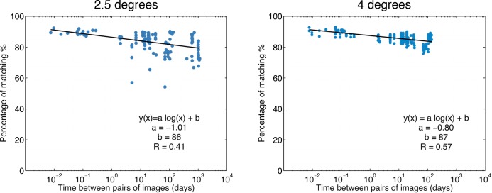
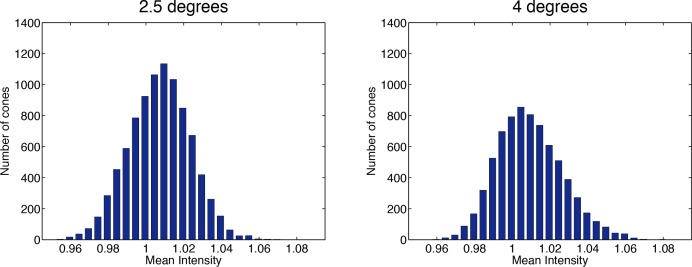
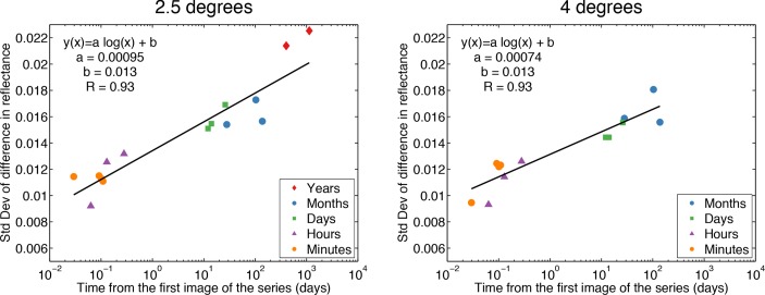
Although there is increasing interest in the investigation of cone reflectance variability, little is understood about its characteristics over long time scales. Cone detection and its automation is now becoming a fundamental step in the assessment and monitoring of the health of the retina and in the understanding of the photoreceptor physiology. In this work we provide an insight into the cone reflectance variability over time scales ranging from minutes to three years on the same eye, and for large areas of the retina (≥ 2.0 × 2.0 degrees) at two different retinal eccentricities using a commercial adaptive optics (AO) flood illumination retinal camera. We observed that the difference in reflectance observed in the cones increases with the time separation between the data acquisitions and this may have a negative impact on algorithms attempting to track cones over time. In addition, we determined that displacements of the light source within 0.35 mm of the pupil center, which is the farthest location from the pupil center used by operators of the AO camera to acquire high-quality images of the cone mosaic in clinical studies, does not significantly affect the cone detection and density estimation.

Keywords: (110.1080) Active or adaptive optics; (170.3880) Medical and biological imaging; (330.7331) Visual optics, receptor optics.

Fig. 1

Screen shot of the anterior segment image of the viewer interface of the AO flood illuminated retinal camera showing the placement of the entry beam (green cross) in the right eye of the subject. The four white dots are the first Purkinje images of the cornea, which are taken by the AO camera operators as reference points for collecting high-quality images of the photoreceptor mosaic. The “on-center” represents the illumination position passing through the center of the pupil; in the “off-center” position, the illumination is 0.35 mm temporal from the pupil center. The corneal reflections allow images of the retina to be captured using the same illumination position over time.

Fig. 2

Example of detection on the same portion of two images obtained from the same frame series. In the upper image, the frames were not corrected for the flat-field prior to registration, in the image below the frames were divided by the flat-field image and then registered. The cone map on the right is the sum of the two cone maps resulting from the separate detections on the two images. The difference between the combined cone map and the two individual cone maps is less than 4% of the cones.

Fig. 3

One frame of the time series at 2.5 degrees after registration and normalization ( Visualization 1). An overview of the data set and the sub-set division is available in Data File 1.

Fig. 4

First frame of the time series at 4.0 degrees after registration and normalization ( Visualization 2). An overview of the data set and the sub-set division is available in Data File 1.

Fig. 5

Detail of detection and segmentation of cones at the same location of a single image (left) and the average image (right). The cones that are detected and segmented on the average image but not on the single image are shown in pink.

Fig. 6

Top row: histograms of the cone intensity in the first and second image of the “Days” series at 2.5 degrees. Bottom: histogram of the difference between the intensity of the cones in the second and the first image fitted with a Gaussian distribution, for which the parameters are shown on the right. These histograms are shown as representative of the results on all the images.

Fig. 7

Flow chart of the entire analysis process. The processing algorithms enclosed in the left and right grey boxes were performed for all the images and for the two series of images at the two retinal locations respectively.

Fig. 8

Average images at 4.0 degrees (left) and 2.5 degrees (right) with the grid of 200 × 200 pixel (160 × 160μm) windows in the image series in which the parameters were calculated. The selected windows are highlighted and marked with numbers. The same numbers are used in the plot legend in Fig. 9.

Fig. 9

Bland-Altman plot of the cone density at 2.5 (circles) and 4.0 degrees (squares) in selected windows. The plot shows the mean of the differences (continuous lines) and ± 1.96 SD (dashed lines) of the cone density between the two illumination positions. The numbers represent the sampling windows shown in Fig. 8.

Fig. 10

Matching of cones performed on pairs of images as a function of the time between the two images, at 2.5 degrees and at 4.0 degrees. The x-axis is in logarithmic scale. The plots show how the percentage of matching decreases as the time increases with a logarithmic trend (linear fits on logarithmic scale).

Fig. 11

Histogram of the mean cone intensity (as measured inside the segmentations) on the average images at 2.5 degrees and 4.0 degrees. The intensity values are measured after the total intensity normalization.

Fig. 12

Standard deviation of the difference in cone reflectance as a function of time at 2.5 degrees and 4.0 degrees. The x-axis is in logarithmic scale. The standard deviation is calculated from the Gaussian fit of the histograms of the intensity difference of all the cones with respect to their intensity value in the first image of the different time series. It can be seen that the variability of cone reflectance increases logarithmically with time (linear fits on logarithmic scale). The variation in cone reflectance between images acquired more than one year apart is more than the double the variation observed on the cone mosaic on the same day.

References

1. Li K. Y., Roorda A., “Automated identification of cone photoreceptors in adaptive optics retinal images,” J. Opt. Soc. Am. A 24, 1358–1363 (2007).10.1364/JOSAA.24.001358 - DOI - PubMed
1. Xue B., Choi S. S., Doble N., Werner J. S., “Photoreceptor counting and montaging of en-face retinal images from an adaptive optics fundus camera,” J. Opt. Soc. Am. A 24, 1364–1372 (2007).10.1364/JOSAA.24.001364 - DOI - PMC - PubMed
1. Lombardo M., Serrao S., Ducoli P., Lombardo G., “Eccentricity dependent changes of density, spacing and packing arrangement of parafoveal cones,” Ophthalmic Physiol. Opt. 33, 516–526 (2013).10.1111/opo.12053 - DOI - PubMed
1. Lombardo M., Serrao S., Lombardo G., “Technical factors influencing cone packing density estimates in adaptive optics flood illuminated retinal images,” PLoS ONE 9, 7402 (2014).10.1371/journal.pone.0107402 - DOI - PMC - PubMed
1. Choi S. S., Doble N., Hardy J. L., Jones S. M., Keltner J. L., Olivier S. S., Werner J. S., “In vivo imaging of the photoreceptor mosaic in retinal dystrophies and correlations with visual function,” Invest. Ophthalmol. Vis. Sci. 47, 2080–2092 (2006).10.1167/iovs.05-0997 - DOI - PMC - PubMed
LinkOut - more resources