Connectome analysis for pre-operative brain mapping in neurosurgery

Abstract

Object: Brain mapping has entered a new era focusing on complex network connectivity. Central to this is the search for the connectome or the brains 'wiring diagram'. Graph theory analysis of the connectome allows understanding of the importance of regions to network function, and the consequences of their impairment or excision. Our goal was to apply connectome analysis in patients with brain tumours to characterise overall network topology and individual patterns of connectivity alterations.

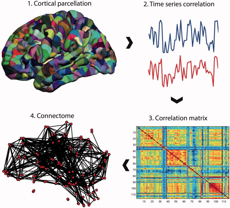
Methods: Resting-state functional MRI data were acquired using multi-echo, echo planar imaging pre-operatively from five participants each with a right temporal-parietal-occipital glioblastoma. Complex networks analysis was initiated by parcellating the brain into anatomically regions amongst which connections were identified by retaining the most significant correlations between the respective wavelet decomposed time-series.

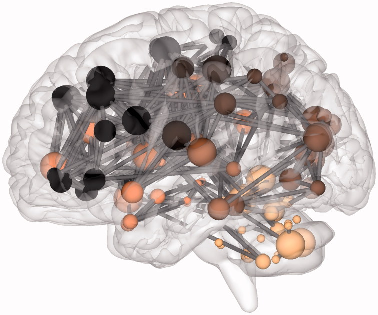
Results: Key characteristics of complex networks described in healthy controls were preserved in these patients, including ubiquitous small world organization. An exponentially truncated power law fit to the degree distribution predicted findings of general network robustness to injury but with a core of hubs exhibiting disproportionate vulnerability. Tumours produced a consistent reduction in local and long-range connectivity with distinct patterns of connection loss depending on lesion location.

Conclusions: Connectome analysis is a feasible and novel approach to brain mapping in individual patients with brain tumours. Applications to pre-surgical planning include identifying regions critical to network function that should be preserved and visualising connections at risk from tumour resection. In the future one could use such data to model functional plasticity and recovery of cognitive deficits.

Keywords: Brain mapping; connectome; echo-planar imaging; glioblastoma; magnetic resonance imaging; neurosurgery.

Figure 1.

Connectome construction. Methods for performing a connectome analysis using resting-state fMRI data as an example, but similar methods can be applied to data acquired from DTI or EEG/MEG. Initially, a template is chosen to divide the brain into different regions (known as parcels) that form the network nodes. These nodes are used to form the rows and columns of a matrix. Entries of the matrix represent edges between each of the nodes and are formed by recording a measure of statistical dependency (such the Pearson correlation co-efficient) between the resting-state fMRI time series of each node. This correlation matrix can then be thresholded and binarised to form an adjacency matrix, although weighted and fully connected matrices (without thresholding) are also possible. Finally, the co-ordinates of each parcel are used to display the node location onto a surface reconstruction of the brain, with edges representing functional connections.

Figure 2.

Effects of thresholding on network degree. Increasing the cut-off of the correlation threshold results in a reduction in the number of edges that survive thresholding in the resulting matrix. The straight black line represents the minimum mean degree for small world networks (n*log(n) = 9.5). The point of intersection of the wavelet scale degree with this line is used as the threshold to form the binary network used for further analysis. Wavelet scales 4 and 5 were not able to produce a matrix of the required mean degree at any threshold and were, therefore, not studied further.

Figure 3.

The connectome in glioblastoma. A sagittal view of an individual patient’s connectome at wavelet scale 2. Nodes are coloured according to their anatomical module (e.g. frontal, central, parietal, etc.) and their size is proportional to their degree. Connections (or edges) are presented in grey and represent the binary entries of the adjacency matrix. Locations are based on the co-ordinates of their original parcels and projected onto a surface reconstruction in MNI space.

Figure 4.

Degree distribution. (A) The histogram for the group network node degrees. The majority of nodes are of low degree (<5) while the maximum degree extends above 30 (although few nodes have this degree). (B) The group network degree distribution is compared to that from simulated networks with either an exponential, power law, or exponentially truncated power law degree distribution. The best fit determined using Akaite Information Criteria was with the exponentially truncated power law degree distribution.

Figure 5.

Random error and targeted attack. The change in the size of the network giant component (top row) or efficiency (bottom row) due to either random error (left column) or targeted attack based on degree centrality (right column). Changes are relative to the values for the intact network. All networks are approximately equally affected by random error. However, targeted attack reveals vulnerability of the scale free network, while the brain network is of intermediate vulnerability between the scale-free and random networks. Horizontal axis values are the proportion of nodes removed and vertical axis values are scaled to maximum. Solid line = brain networks, dotted line = simulated scale-free networks, dashed line = simulated random networks

Figure 6.

Brain mapping with graph theory network measures. Axial view of node features displayed in cortical surface reconstructions. (A) Node size is proportional to clustering co-efficient. (B) Node size is proportional to information centrality. In both figures, those nodes that are spatially adjacent to the tumour are highlighted. Network edges are removed to focus on the node features. If one were to use this information for pre-surgical planning, purposefully sacrificing selected smaller nodes to allow an extended surgical resection could be seen as having a minimal effect on overall network efficiency (and, therefore, by extrapolation on higher cognitive features such as intelligence). However, inadvertently affecting too many of larger nodes would be expected to have a disproportionate effect on overall network efficiency, and, therefore, should be avoided.

Figure 7.

Connections at risk. Circular representations of brain functional connectivity data (individual patient data, wavelet scale 2). Images are in neurological projection (image left = left hemisphere) with superior aspect of the image representing anterior brain (akin to an axial view). The sides are symmetrical representations of individual lobes (and parcels within) in their anterior–posterior co-ordinates. Inner circular heatmaps represent degree, clustering, and information centrality (outside to inside) per parcel. Lines representing intra-lobe connections are outside with inter-lobe connections in the centre. On the right, the nodes closest to the tumour are highlighted in red, while on the left the homologous nodes from the contralateral hemisphere are shown for comparison. The tumour was associated with reduced connectivity at intra-lobar, intra-hemispheric and inter-hemispheric levels. These effects were clear and consistent at the individual participant level. If one were to use this for tumour planning, then the connections in red would represent those that could be affected by extending the resection outside of the contrast enhancing margin, and would then become ‘connections at risk’. Parcel codes (alphabetical): ACIN: anterior cingulate; AG: angular gyrus; AMYG: amygdala; CAU: caudate; CHB: biventricular; CHCL: central lobule; CHCU: culmen; CHF: floculus; CHG: gracilis; CHIS: inferior semilunar; CVL: lingual; CHS: simplex; CHSS: superior semilunar; CHT: tonsil; CV: vermis; F1M: superior medial frontal; F1MO: superior frontal medial orbital; F2: middle frontal; F20: middle orbital; F30: inferior frontal pars orbitalis; F3OP: inferior frontal pars opercularis; F3T: inferior frontal pars triangularis; FUSI: fusiform; GR: gyrus recturs; HES: Heschl gyrus; HIP: hippocampus; IFG: inferior frontal gyrus; IN: insula; LING: lingual; MCIN: middle cingulate; O1: inferior occipital; O2: middle occipital; O3: superior occipital; OC: olfactory cortex; P1: superior parietal lobule; P2: inferior parietal lobule; PAL: lentiform nucleus; PCIN: posterior cingulate; PCL: paracentral lobule; PHIP: parahippocampal gyrus; POST: post-central; PRE: precentral; PQ: precuneus; PUT: putamen; Q: cuneus; RO: rolandic operculum; SMA: supplementary motor area; SMG: supramarginal gyrus; T1: superior temporal; T1P: temporal pole; T2: middle temporal; T2P: middle temporal pole; T3: inferior temporal; THA: thalamus; V1: calcarine.

Figure 7.

Connections at risk. Circular representations of brain functional connectivity data (individual patient data, wavelet scale 2). Images are in neurological projection (image left = left hemisphere) with superior aspect of the image representing anterior brain (akin to an axial view). The sides are symmetrical representations of individual lobes (and parcels within) in their anterior–posterior co-ordinates. Inner circular heatmaps represent degree, clustering, and information centrality (outside to inside) per parcel. Lines representing intra-lobe connections are outside with inter-lobe connections in the centre. On the right, the nodes closest to the tumour are highlighted in red, while on the left the homologous nodes from the contralateral hemisphere are shown for comparison. The tumour was associated with reduced connectivity at intra-lobar, intra-hemispheric and inter-hemispheric levels. These effects were clear and consistent at the individual participant level. If one were to use this for tumour planning, then the connections in red would represent those that could be affected by extending the resection outside of the contrast enhancing margin, and would then become ‘connections at risk’. Parcel codes (alphabetical): ACIN: anterior cingulate; AG: angular gyrus; AMYG: amygdala; CAU: caudate; CHB: biventricular; CHCL: central lobule; CHCU: culmen; CHF: floculus; CHG: gracilis; CHIS: inferior semilunar; CVL: lingual; CHS: simplex; CHSS: superior semilunar; CHT: tonsil; CV: vermis; F1M: superior medial frontal; F1MO: superior frontal medial orbital; F2: middle frontal; F20: middle orbital; F30: inferior frontal pars orbitalis; F3OP: inferior frontal pars opercularis; F3T: inferior frontal pars triangularis; FUSI: fusiform; GR: gyrus recturs; HES: Heschl gyrus; HIP: hippocampus; IFG: inferior frontal gyrus; IN: insula; LING: lingual; MCIN: middle cingulate; O1: inferior occipital; O2: middle occipital; O3: superior occipital; OC: olfactory cortex; P1: superior parietal lobule; P2: inferior parietal lobule; PAL: lentiform nucleus; PCIN: posterior cingulate; PCL: paracentral lobule; PHIP: parahippocampal gyrus; POST: post-central; PRE: precentral; PQ: precuneus; PUT: putamen; Q: cuneus; RO: rolandic operculum; SMA: supplementary motor area; SMG: supramarginal gyrus; T1: superior temporal; T1P: temporal pole; T2: middle temporal; T2P: middle temporal pole; T3: inferior temporal; THA: thalamus; V1: calcarine.

Figure 7.

Connections at risk. Circular representations of brain functional connectivity data (individual patient data, wavelet scale 2). Images are in neurological projection (image left = left hemisphere) with superior aspect of the image representing anterior brain (akin to an axial view). The sides are symmetrical representations of individual lobes (and parcels within) in their anterior–posterior co-ordinates. Inner circular heatmaps represent degree, clustering, and information centrality (outside to inside) per parcel. Lines representing intra-lobe connections are outside with inter-lobe connections in the centre. On the right, the nodes closest to the tumour are highlighted in red, while on the left the homologous nodes from the contralateral hemisphere are shown for comparison. The tumour was associated with reduced connectivity at intra-lobar, intra-hemispheric and inter-hemispheric levels. These effects were clear and consistent at the individual participant level. If one were to use this for tumour planning, then the connections in red would represent those that could be affected by extending the resection outside of the contrast enhancing margin, and would then become ‘connections at risk’. Parcel codes (alphabetical): ACIN: anterior cingulate; AG: angular gyrus; AMYG: amygdala; CAU: caudate; CHB: biventricular; CHCL: central lobule; CHCU: culmen; CHF: floculus; CHG: gracilis; CHIS: inferior semilunar; CVL: lingual; CHS: simplex; CHSS: superior semilunar; CHT: tonsil; CV: vermis; F1M: superior medial frontal; F1MO: superior frontal medial orbital; F2: middle frontal; F20: middle orbital; F30: inferior frontal pars orbitalis; F3OP: inferior frontal pars opercularis; F3T: inferior frontal pars triangularis; FUSI: fusiform; GR: gyrus recturs; HES: Heschl gyrus; HIP: hippocampus; IFG: inferior frontal gyrus; IN: insula; LING: lingual; MCIN: middle cingulate; O1: inferior occipital; O2: middle occipital; O3: superior occipital; OC: olfactory cortex; P1: superior parietal lobule; P2: inferior parietal lobule; PAL: lentiform nucleus; PCIN: posterior cingulate; PCL: paracentral lobule; PHIP: parahippocampal gyrus; POST: post-central; PRE: precentral; PQ: precuneus; PUT: putamen; Q: cuneus; RO: rolandic operculum; SMA: supplementary motor area; SMG: supramarginal gyrus; T1: superior temporal; T1P: temporal pole; T2: middle temporal; T2P: middle temporal pole; T3: inferior temporal; THA: thalamus; V1: calcarine.

References

1. Greenblatt SH, Dagi TF, Epstein MH, editors. A history of neurosurgery: in its scientific and professional contexts. Park Ridge, IL: AANS; 1997.
1. Penfield W, Rasmussen T. The cerebral cortex of man. New York: Macmillan; 1950.
1. Fornito A, Zalesky A, Breakspear M. Graph analysis of the human connectome: promise, progress, and pitfalls. NeuroImage. 2013;80:426–44. - PubMed
1. Smith SM, Beckmann CF, Andersson J.et al.Resting-state fMRI in the human connectome project. NeuroImage 201380144–68. - PMC - PubMed
1. Sporns O, editor. Discovering the human connectome. USA: MIT Press; 2012.
MeSH terms
LinkOut - more resources