Deep learning for computational biology

Abstract

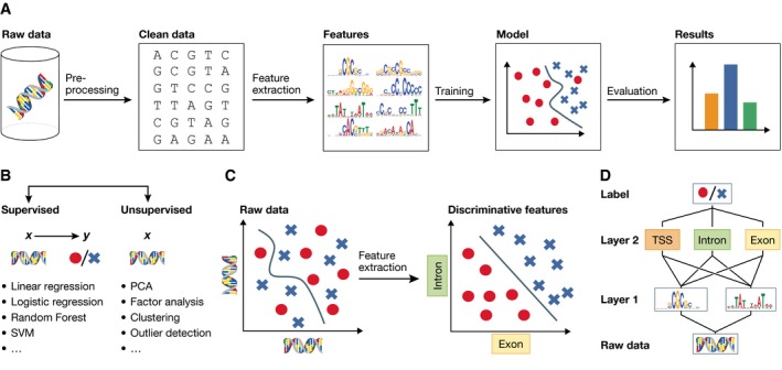
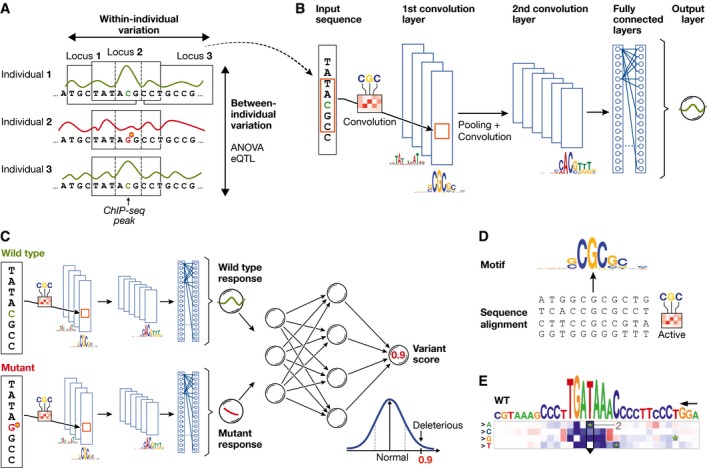
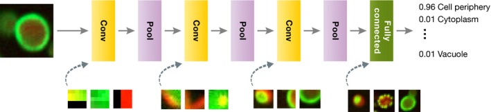
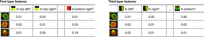
Technological advances in genomics and imaging have led to an explosion of molecular and cellular profiling data from large numbers of samples. This rapid increase in biological data dimension and acquisition rate is challenging conventional analysis strategies. Modern machine learning methods, such as deep learning, promise to leverage very large data sets for finding hidden structure within them, and for making accurate predictions. In this review, we discuss applications of this new breed of analysis approaches in regulatory genomics and cellular imaging. We provide background of what deep learning is, and the settings in which it can be successfully applied to derive biological insights. In addition to presenting specific applications and providing tips for practical use, we also highlight possible pitfalls and limitations to guide computational biologists when and how to make the most use of this new technology.

Keywords: cellular imaging; computational biology; deep learning; machine learning; regulatory genomics.

Figure 1. Machine learning and representation learning

(A) The classical machine learning workflow can be broken down into four steps: data pre‐processing, feature extraction, model learning and model evaluation. (B) Supervised machine learning methods relate input features x to an output label y, whereas unsupervised method learns factors about x without observed labels. (C) Raw input data are often high‐dimensional and related to the corresponding label in a complicated way, which is challenging for many classical machine learning algorithms (left plot). Alternatively, higher‐level features extracted using a deep model may be able to better discriminate between classes (right plot). (D) Deep networks use a hierarchical structure to learn increasingly abstract feature representations from the raw data.

Figure 2. Principles of using neural networks for predicting molecular traits from DNA sequence

(A) DNA sequence and the molecular response variable along the genome for three individuals. Conventional approaches in regulatory genomics consider variations between individuals, whereas deep learning allows exploiting intra‐individual variations by tiling the genome into sequence DNA windows centred on individual traits, resulting in large training data sets from a single sample. (B) One‐dimensional convolutional neural network for predicting a molecular trait from the raw DNA sequence in a window. Filters of the first convolutional layer (example shown on the edge) scan for motifs in the input sequence. Subsequent pooling reduces the input dimension, and additional convolutional layers can model interactions between motifs in the previous layer. (C) Response variable predicted by the neural network shown in (B) for a wild‐type and mutant sequence is used as input to an additional neural network that predicts a variant score and allows to discriminate normal from deleterious variants. (D) Visualization of a convolutional filter by aligning genetic sequences that maximally activate the filter and creating a sequence motif. (E) Mutation map of a sequence window. Rows correspond to the four possible base pair substitutions, columns to sequence positions. The predicted impact of any sequence change is colour‐coded. Letters on top denote the wild‐type sequence with the height of each nucleotide denoting the maximum effect across mutations (figure panel adapted from Alipanahi et al, 2015).

Figure 3. Convolution and pooling operators are stacked, thereby creating a deep network for image analysis

In standard applications, convolution layers are followed by a pooling layer (Box 2). In this example, the lowest level convolutional units operate on 3 × 3 patches, but deeper ones use and capture information from larger regions. These convolutional pattern‐matching layers are followed by one or multiple fully connected layers to learn which features are most informative for classification. For each layer with learnable weights, three example images that maximize some neuron output are shown.

Figure 4. A pre‐trained network can be used as a generic feature extractor

Feeding input into the first layer (left) gives a low‐level feature representation in terms of patterns (left to right) present in smaller patches in every cell (top to bottom). Neuron activations extracted from deeper layers (right) give rise to more abstract features that capture information from a larger segment of the image.

Figure 5. Data normalization for and pre‐processing for deep neural networks

(A) DNA sequence one‐hot encoded as binary vectors using codes A = 1 0 0 0, G = 0 1 0 0, C = 0 0 1 0 and T = 0 0 0 1. (B) Continuous data (green) after zero‐centring (orange), scaling to unit variance (blue) and whiting (purple). (C) Holdout validation partitions the full data set randomly into training (~60%), validation (~10%) and test set (~30%). Models are trained with different hyper‐parameters on the training set, from which the model with the highest performance on the validation set is selected. The generalization performance of the model is assessed and compared with other machine learning methods on the test set. (D) The shape of the learning curve indicates if the learning rate is too low (red, shallow decay), too high (orange, steep decay followed by saturation) or appropriate for a particular learning task (green, gradual decay). (E) Large differences in the model performance on the training set (blue) and validation set (green) indicate overfitting. Stopping the training as soon as the validation set performance starts to drop (early stopping) can prevent overfitting. (F) Illustration of the dropout regularization. Shown is a feedforward neural network after randomly dropping out neurons (crossed out), which reduces the sensitivity of neurons to neurons in the previous layer due to non‐existent inputs (greyed edges).

References

1. Abadi M, Agarwal A, Barham P, Brevdo E, Chen Z, Citro C, Corrado GS, Davis A, Dean J, Devin M, Ghemawat S, Goodfellow I, Harp A, Irving G, Isard M, Jia Y, Josofowicz R, Kaiser L, Kudlur M, Levenberg J et al (2016) TensorFlow: large‐scale machine learning on heterogeneous distributed systems. arXiv:1603.04467
1. Agathocleous M, Christodoulou G, Promponas V, Christodoulou C, Vassiliades V, Antoniou A (2010) Protein secondary structure prediction with bidirectional recurrent neural nets: can weight updating for each residue enhance performance? In Artificial Intelligence Applications and Innovations, Papadopoulos H, Andreou AS, Bramer M. (eds), Vol. 339, pp 128–137. Berlin Heidelberg: Springer;
1. Alain G, Bengio Y, Rifai S (2012) Regularized auto‐encoders estimate local statistics. In Proc. CoRR, pp 1–17
1. Albert FW, Treusch S, Shockley AH, Bloom JS, Kruglyak L (2014) Genetics of single‐cell protein abundance variation in large yeast populations. Nature 506: 494–497 - PMC - PubMed
1. Alipanahi B, Delong A, Weirauch MT, Frey BJ (2015) Predicting the sequence specificities of DNA‐ and RNA‐binding proteins by deep learning. Nat Biotechnol 33: 831–838 - PubMed
Publication types