Analysis of Neuronal Spike Trains, Deconstructed

Abstract

As information flows through the brain, neuronal firing progresses from encoding the world as sensed by the animal to driving the motor output of subsequent behavior. One of the more tractable goals of quantitative neuroscience is to develop predictive models that relate the sensory or motor streams with neuronal firing. Here we review and contrast analytical tools used to accomplish this task. We focus on classes of models in which the external variable is compared with one or more feature vectors to extract a low-dimensional representation, the history of spiking and other variables are potentially incorporated, and these factors are nonlinearly transformed to predict the occurrences of spikes. We illustrate these techniques in application to datasets of different degrees of complexity. In particular, we address the fitting of models in the presence of strong correlations in the external variable, as occurs in natural sensory stimuli and in movement. Spectral correlation between predicted and measured spike trains is introduced to contrast the relative success of different methods.

Keywords: dimensional reduction; feature vector; neuroinformatics; predictive modeling; reverse correlation; systems identification; time series.

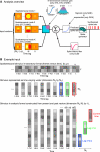
Figure 1. Schematic for the Generation of Spike Trains from Stimuli from Different Classes of Models

(A) An LN model consists of a number of processing steps that transform the input stimulus into a predicted spike train. Here we illustrate the types of processing stages included in the computational methods we consider. Most generally, the stimulus is projected onto one or more features and may then be passed through a nonlinear function whose dimensionality is given by the number of features. The result of this may be summed with a term that depends on the spike history and passed through a further nonlinear function. Finally there is a stochastic spike generation mechanism that yields a spike train. None of the methods we will consider have all model components; one should choose among the methods depending on the nature of the stimulus, the type of response, and the need for parsimony. For example, only the generalized linear model includes the influence of the spike history. (B) Here we illustrate how an example visual stimulus is reformatted as a time-dependent vector. Each stimulus frame has two spatial coordinates and a total of N_X pixels. First, the frame presented in each time point is unwrapped to give a N_X-dimensional vector. Then, if the model we will construct depends on the stimulus at N_T time points, the final stimulus is a vector in which the spatial component is copied across consecutive time points to form N = N_X×N_T components.

Figure 2. Schematic of Stimulus Samples Plotted in Two Arbitrary Directions in Stimulus Space as Gray and Red Dots

(A–C) Only red dots lead to a spike. (A) The STA is a vector that points to the mean of the spike-triggered stimuli (red dots). (B) The covariance of the spike-triggered stimuli captures the coordinates of variation of the cloud. The covariance of the stimulus, i.e., the underlying stimulus covariance C_p (solid gray circle), forms one set of vectors, and the covariance of the spike-triggered stimuli, C_s, forms a second set. The two dominant vectors comprising their difference, i.e., ΔC = C_s - C_p, yield the dominant STC two modes. The mode is significant only if its length is larger than the radius of the underlying stimulus covariance. (C) The naively computed STA for the case of correlated or colored noise, where the variance of the underlying stimulus distribution is heterogeneous.

Figure 3. Spike Responses from Salamander Retinal Ganglion Cell 3 for a Visual Checkerboard Stimulus, Used to Illustrate the Methods with a “White Noise” Stimulus

(A) Each pixel in the checkerboard was refreshed each Δt = 33.33 ms with a random value, and the spikes were recorded within the same interval. (B) We constructed the covariance matrix of the stimulus (Equation 18) and plotted its spectrum (black). The eigenvalues are all close to the variance of a single pixel, σ² = 1, for the checkerboard stimulus. We compared this spectrum to that expected theoretically for the same-sized random matrix (Marčenko and Pastur, 1967) with signal-to-noise parameter γ = n/N (number of samples divided by number of dimensions). (C) The hallmark of white noise is that there is no structure in the stimulus, and indeed the eigenvectors of the stimulus covariance matrix (Equation 18) that correspond to the largest eigenvalues are seen to contain no spatial or temporal structure. Methods: The dataset consists of 53 time series of spike arrival times simultaneously recorded from 53 retinal ganglion cells of retinae that had been isolated from larval tiger salamander (Ambystoma tigrinum) and laid upon a square array of planar electrodes (Segev et al., 2004). The pitch of the array was 30 μm and the spiking output of each cell, which includes spikes in both the soma and the axon, was observed on several electrodes. Using a template distributed across multiple electrodes enables one to accurately identify spikes as arising from a single retinal ganglion cell. Visual stimuli were a 40² = 1600 square pixel array that was displayed on a cathode ray tube monitor at a frame rate of 30 Hz (Segev et al., 2006). Each pixel was randomly selected to be bright or dark relative to a mean value on each successive frame, i.e., the amplitude of each pixel was distributed bimodally and was spectrally white up to the Nyquist frequency of 15 Hz. The image from the monitor was conjugate with the plane of the retina and the magnification was such that visual space was divided into 50 μm squares on the retina, which allowed many squares to fit inside the spatial receptive field of each ganglion cell, with a cut-off of 200 cm⁻¹ in spatial frequency. For each cell, we extracted either the 14² = 196 or the 10² = 100 pixel region with modulated activity; these give rise to 2¹⁹⁶ or 2¹⁰⁰ potential patterns, respectively. Each time series was 60–120 min long and contained between 1,000 and 10,000 spikes, but samples a tiny fraction of the potential patterns.

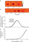
Figure 4. The Spike-Triggered Average ϕ_sta, for the Responses of Retinal Ganglion Cell 3

(A and B) We considered two stimulus representations. In (A), we show a short sequence where we retain three stimulus frames in the past (N_T = 3), and the frame was N_X = 14² = 196 pixels. We chose the optimal lag for which the cell's response is maximally modulated by the stimulus. In (B), we show a long sequence where N_T = 6, but the frame was cropped such that N_X = 10×10 = 100. We chose the first six frames into the past. (C) The underlying stimulus distribution computed for both representations, (A) and (B), in solid and dashed curves, respectively. (D) The expectation procedure (Equations 6 and 7) was used to obtain the input/output nonlinearity for both representations, (A) and (B), in solid and dashed curves, respectively.

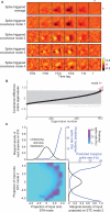
Figure 5. The Spike-Triggered Covariance Features for the Response of Retinal Ganglion Cell 3

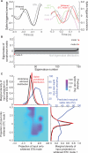
(A) The two significant STC feature vectors, in addition to the STA feature for comparison, using the stimulus representation with N_T = 6 and N_X = 100. The feature vector ϕ_stc,1 has 0.93 overlap with ϕ_sta, while ϕ_stc,2 through ϕ_stc,4 have only a 0.20, 0.11, and a 0.05 overlap, respectively. (B) The significance of each candidate STC feature, i.e., eigenvectors of ΔC (Equation 20), were determined by comparing the corresponding eigenvalue (red and black) to the null distribution (gray shaded area). We used 1,000 repetitions of the calculation for randomized spike trains, corresponding to a confidence interval of 0.001. (C) The nonlinearity in the space spanned by the STA and the second orthogonalized STC feature, after the STA feature was projected out (Equation 24), ${\varphi }_{\mathrm{stc},2}^{\perp }$, completes the construction of the spiking model. The nonlinearity is found by the expectation procedure (Equations 6 and 7). The marginals of this distribution give nonlinearities with respect to the STA (top) and second STC features (right) alone.

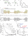
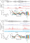
Figure 6. Spike Responses from Thalamic Cell 57 in Response to Whisking in Air without Contact

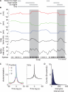
(A) The coordinate systems used to describe the whisk cycle. The left is absolute angle, θ_whisk, and the right is phase, Φ(t), which are related by θ_whisk(t) = θ_protract – θ_amp(1 – cos(Φ(t))) (Deschênes et al., 2016). (B) The spike rate as a function of phase in the whisk cycle. The peak defines the preferred phase Φ_o. (C) A typical whisk, the stimulus, and spikes in the vibrissa area of ventral posterior medial thalamus. We show raw whisking data and, as a check, the data after the slowly varying components θ_protract and θ_amp and the rapidly varying component Φ(t) were found by the Hilbert trasform and the whisk reconstructed. (D) Reconstructed whisk, leaving out slowly varying mid-point θ_protract – θ_amp. The self-motion stimulus is taken as the vibrissa position up to 300 ms in the past with Δt = 2 ms time bins, so that N_x = 1, N_T = 150, and thus N = 150. (E) The spectrum of the covariance matrix of the self-motion (Equation 18). Note the highly structured dominant modes. (F) The inter-whisk and inter-spike intervals. (G) The autocorrelation of whisking. Black is over all trials and gray is only over large amplitude whisks. Note the narrow band nature of this dataset. Methods: The whisking dataset is used to illustrate our methods with a stimulus that contains strong temporal correlations. It consists of seven sets of spike arrival times, each recorded from a single unit in the vibrissa region of ventral posterior medial thalamus of awake, head-restrained rats (Moore et al., 2015b). The animals were motivated to whisk by the smell of their home cage. Spiking data were obtained with quartz pipets using juxtacellular recording (Moore et al., 2015a); this method ensures that the spiking events originate from a single cell. The anterior-to-posterior angle of the vibrissae as a function of time was recorded simultaneously using high-speed videography. Each time series contained 4–14 trials, each 10 s in length, with between 1,300 and 3,500 spikes per time series. The correlation time of the whisking, which serves as the stimulus for encoding by neurons in thalamus, is nominally 0.2 s (Hill et al., 2011a). We found that the cells’ response was strongly modulated by the dynamics of vibrissa motion only when the amplitude θ_amp was relatively high; therefore we constructed the models and tested their predictions only for periods when θ_amp≥10°.

Figure 7. The Spike-Triggered Average and Spike-Triggered Covariance Feature Vectors for the Response of Thalamic Cell 57 in the Rat Vibrissa System

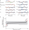
(A) The STA feature and the same feature computed for the whitened stimulus, along with the leading STC features calculated with and without whitening. The dashed curves are after projecting out the STA vector from the STC modes. (B) Comparing the eigenvalues of ΔC, without whitening, to the null eigenvalue distribution computed from randomly shifted spike trains demonstrates the statistical significance of the leading STC eigenvectors; red denotes significant eigenvectors and black not significant. For the case of ΔC with whitening, regularization led to only three eigenvectors, of which one was significant. (C) A two-dimensional model of the nonlinearity for ${\widehat{\varphi }}_{\mathrm{sta}}$ and the leading STC feature, ${\widehat{\varphi }}_{\mathrm{stc},1}$, both computed after whitening. We further plot the two marginals.

Figure 8. The Dominant Features Calculated by the Maximum Noise Entropy Method for Example Thalamic Cell 57

(A) We fit a MNE model to the spike train with the same stimulus representation, with N = 150, and plot the first feature, i.e., h, and statistically significant second-order feature vectors, i.e., eigenvectors of J (Equation 34). We also plot the STA feature next to the first-order mode for comparison. (B) The number of significant second-order features was found by comparing the eigenvalues of J to a null distribution.

Figure 9. The Fit of the Generalized Linear Model for the Responses of Retina Ganglion Cell 3 and Thalamic Vibrissa Cell 57

(A and C) The stimulus feature ϕ_glm compared with the previously calculated STA feature. (B and D) The spike history filters ψ (black curves) along with the exponent of the filter (gray).

Figure 10. Summary of the Performance of Model Predictions for the Retinal Ganglion Cell 3

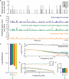
(A–F) Three methods—STA, STC plus STA, and GLM—are compared. (A) A part of the spike train cut out from the test set for illustration purposes. Insert: expanded temporal scale to highlight the slight delay inherent with the GLM. (B) The predicted spike count per frame obtained by computing the probability of a spike corresponding to each stimulus frame (top, STA; middle, STC; bottom, GLM). Note that to generate a prediction from the GLM at time t we need the history of the spike train up to that point t′ < t, which is not deterministic due to the Poisson variability. Thus, the trace presented here (orange) is the average spike count over 500 simulations of the GLM on the test set. (C) The log-likelihood (Equation 47) of each model given the test set, which quantifies the quality of the prediction. We further include the log-likelihood for the null condition (Equation 48). The bars are one standard error jack-knife estimates. (D) The spectral power of individual pixels in the stimulus (black) and the recorded spike train (gray), as well as those of the predicted spike trains. The mean value has been removed, so that the initial data point represents an average over the spectral half-bandwidth. Spectra were computed with a half-bandwidth of 0.087 Hz as an average over 159 spectral estimators for 920 s of data. (E) The phase and magnitude of the spectral coherence between the recorded and predicted spike train for each method. Coherence was computed with a half-bandwidth of 0.065 Hz as an average over 119 spectral estimators. (F) The coherence averaged from 0.5 to 5.0 Hz, together with one standard error jack-knife estimates for the average.

Figure 11. Summary of the Performance of Predicted Spike Trains for Thalamic Neuron 57

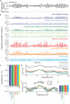
(A–F) Seven means of analysis are compared, i.e., STA, STA after whitening of the stimulus, STC plus STA, STA and STC after whitening of the stimulus, MNE, GLM, and a phase tuning curve model. (A) The stimulus corresponds to vibrissa position with slowly carrying changes in the set-point removed. (B) The predicted probability of spiking per 2 ms time bin obtained by computing by each model and the corresponding stimulus. Note that to generate a prediction from the GLM at time t, we need the history of the spike train up to that point, t′ < t, which is not deterministic due to the Poisson variability. Thus, the trace presented here (orange) is the average spike count over 500 simulations of the GLM on the test set. (C) The log-likelihood (Equation 47) of each model given the test set, which quantifies the quality of the prediction. The bars are one standard error computed as a jack-knife estimate. (D) The power spectra of individual pixels in the stimulus (black) and the recorded spike train (gray), as well as those of the predicted spike trains. Spectra were computed with a half-bandwidth of 0.6 Hz as an average over 23 spectral estimators. (E) The phase and magnitude of the coherence between the recorded and predicted spike train for each method (Equation 49). Coherence was computed with a half-bandwidth of 1.2 Hz as an average over 49 spectral estimators. (F) The magnitude of the coherence at the peak of the spectrum for whisking (*), 6.7 Hz, with one standard error jack-knife estimates.

Figure 12. Summary of the Performance of Predicted Spike Trains for Two Additional Thalamic Cells, Units 88 and 99

(A–E) The whisking stimulus (A) and predicted spike probabilities (B) for a cell with weak phase tuning (C). Yet this cell was strongly modulated by the amplitude of whisking, which changes on a slow timescale, approximately 1 s, compared with changes in phase. The predicted rate is shown for two models that perform best, i.e., STA after whitening of the stimulus and MNE. The phase tuning model performs poorly as it ignores the amplitude (D). The one standard error jack-knife was calculated for the coherence at low frequency (*), 0.5 Hz (E). (F–J) The whisking stimulus (F) and predicted spike probabilities (G) for a cell with particularly strong phase tuning (H). The predicted rate is shown for three models that perform best, i.e., STA after whitening of the stimulus, MNE, and the phase tuning model. Here the coherence between the predictions and the measurements in the whisking frequency band is near 1.0 for all models (I). The one standard error jack-knife was calculated for the coherence at low frequency (*), 0.5 Hz (J).

Figure 13. Summary of the Three-Dimensional Monkey-Based Reach Task with Spike Data from Unit 36

(A–D) Analysis is based on a single ~90 min recording session in which the monkey performed the task; both cursor motion and grip force are recorded. (A) Grip-and-reach task involves first moving the cursor to a central position, followed by gripping the handle with sufficient force. Once gripping at the center, after a variable wait time, a target appears randomly in one of eight locations. Following another wait of a variable time, the cue at the origin disappears, acting as a go signal, after which the monkey may perform the reach movement. Grip on the handle has to be maintained through the duration of the trial. A successful trial requires reaching the target within a set time limit. Once the target is reached, the monkey needs to hold the cursor at the target for 700 ms and to release its grip on the handle. Following a successful trial, the monkey receives a reward, and after an inter-trial period, the next trial begins. (B) Measured cursor position and grip force. (C) Stimulus autocorrelation. (D) Distribution of inter-spike intervals shows a clear refractory period. Methods: Spikes were recorded from single isolated units in the contralateral cortex to the task arm using an intracortical multi electrode array (Blackrock Utah array) implanted in the arm region of M1. Spiking data were binned into millisecond intervals, while both cursor data and grip force are sampled at 100 Hz. Of the isolated units, we selected those that showed no evidence of contamination based on inspection of the inter-spike interval distribution. Analysis was performed from the time of the Go signal until the grip was released; see gray band in (B).

Figure 14. Network GLM Features and Validation for Monkey Reach Data Using the Interval between the Start of the Go Signal and the End of the Trial

(A) Spike history filter for sample unit 36, one of nine concurrently recorded units in our analysis. The nine were chosen as those out of 45 units with no extra spikes in the refractory period of the inter-spike interval. Red curve shows result for the coupled model (κ = 100 in 52), and black curve shows the filter in the absence of coupling between units; in this case the two curves are indistinguishable. (B) Spike history filters from eight neighboring cells for the coupled model (κ = 100). The coupling terms are non-zero for three neighbors. (C) Feature vectors calculated for the network, i.e., coupled (red), and single cell, i.e., uncoupled GLM (black). (D) Scatterplot of log-likelihood between predicted spike rate and observed spike train for the coupled and uncoupled model. The red dot refers to the data in (A)–(C); the bars are one standard error jack-knife estimates. (E) The spectral coherence, calculated as an average over all trials with a 0.5 Hz bandwidth, for the network, i.e., coupled (red), and single cell, i.e., uncoupled GLM (black). The band is one standard error. (F) Scatterplot of the coherence between predicted spike rate and observed spike train for the coupled and uncoupled models. The ellipses are one standard error jack-knife estimates. The red ellipse refers to the data in (A)–(C) and (E). The red and blue data are significant at the level of three standard errors (0.01), the green data barely significant at two standard errors (0.05), and the gray data have no significant improvement from coupling to the network.

Figure B3. Two-Dimensional Vector Plots

(A) Example vectors. (B) Eigenvectors of our example matrix M. Each has unit length.

References

1. Adelman TL, Bialek W, Olberg RM. The information content of receptive fields. Neuron. 2003;40:823–833. - PubMed
1. Agüera y Arcas B, Fairhall AL. What causes a neuron to spike? Neural Comput. 2003;15:1789–1807. - PubMed
1. Akaike H. Information theory as an extension of the maximum likelihood principle. In: Petrov BN, Caski F, editors. Proceeding of the Second International Symposium on Information Theory. Akademiai Kiado; 1973. pp. 267–281.
1. Alivisatos AP, Chun M, Church GM, Greenspan RJ, Roukes ML, Yuste R. The brain activity map project and the challenge of functional connectomics. Neuron. 2012;74:970–974. - PMC - PubMed
1. Aljadeff J, Segev R, Berry MJ, 2nd, Sharpee TO. Spike triggered covariance in strongly correlated gaussian stimuli. PLoS Comput. Biol. 2013;9:e1003206. - PMC - PubMed
Publication types