A review on regional convection-permitting climate modeling: Demonstrations, prospects, and challenges

Abstract

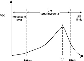
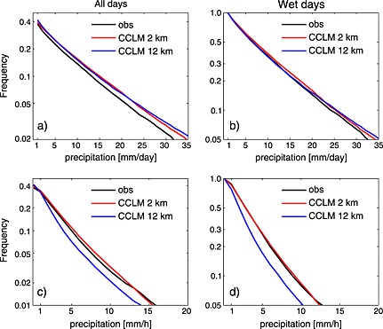
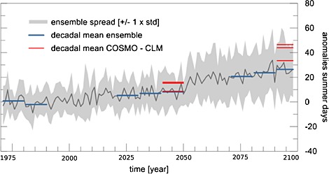
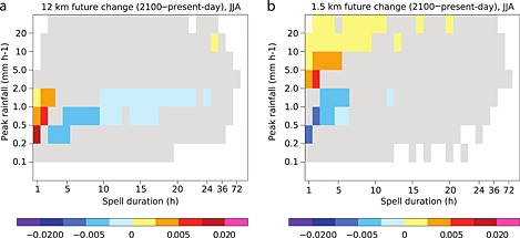
Regional climate modeling using convection-permitting models (CPMs; horizontal grid spacing <4 km) emerges as a promising framework to provide more reliable climate information on regional to local scales compared to traditionally used large-scale models (LSMs; horizontal grid spacing >10 km). CPMs no longer rely on convection parameterization schemes, which had been identified as a major source of errors and uncertainties in LSMs. Moreover, CPMs allow for a more accurate representation of surface and orography fields. The drawback of CPMs is the high demand on computational resources. For this reason, first CPM climate simulations only appeared a decade ago. In this study, we aim to provide a common basis for CPM climate simulations by giving a holistic review of the topic. The most important components in CPMs such as physical parameterizations and dynamical formulations are discussed critically. An overview of weaknesses and an outlook on required future developments is provided. Most importantly, this review presents the consolidated outcome of studies that addressed the added value of CPM climate simulations compared to LSMs. Improvements are evident mostly for climate statistics related to deep convection, mountainous regions, or extreme events. The climate change signals of CPM simulations suggest an increase in flash floods, changes in hail storm characteristics, and reductions in the snowpack over mountains. In conclusion, CPMs are a very promising tool for future climate research. However, coordinated modeling programs are crucially needed to advance parameterizations of unresolved physics and to assess the full potential of CPMs.

Keywords: added value; climate; cloud resolving; convection‐permitting modeling; high resolution; nonhydrostatic modeling.

Figure 1

Visualization of four different modeling approaches for convection‐permitting climate simulations: (a) limited‐area modeling, (b) global CPM climate simulations, (c) superparameterizations, and (d) stretched‐grid models.

Figure 2

(a–p) Summary of the domains (schematic) used in the different CPM climate simulations that are addressed in this paper. The acronyms are defined in Table 1.

Figure 3

The behavior of a convection‐permitting simulation across kilometer‐scale grid spacings is illustrated for the example of orographic convection over the southwestern parts of the European Alps. (a) Snapshots of the cloud liquid water content of clouds within a 350 km × 350 km large subdomain of the full modeling domain. The increase in resolution decreases the size of individual clouds and increases the number of convective clouds. (b) The surface rain rate averaged over a larger domain covering the whole Alpine mountain range. (c) The 9 day average diurnal cycle obtained from the time series shown in Figure 3b. The magnitude and timing of surface precipitation are largely insensitive to the horizontal grid spacing (adapted from Langhans et al. [2012a], ©Copyright 2012 American Meteorological Society (AMS)).

Figure 4

Vertical velocity in an idealized linearly sheared flow passed a quasi 2‐D hill with the nonhydrostatic (a) EULAG model and the corresponding (b) nonhydrostatic and (c) hydrostatic IFS simulations [Wedi and Smolarkiewicz, 2009]. IFS is the numerical model used at ECMWF, Reading, for midrange and seasonal forecasts. As demonstrated here, the hydrostatic version of IFS fails to simulate horizontally propagating gravity waves and the need for nonhydrostatic formulations becomes obvious. “©[2010 ECMWF]” Copyright belongs to the European Centre for Medium‐Range Weather Forecasting (ECMWF).

Figure 5

Simplified turbulence spectrum ϕ(κ) as a function of the horizontal wave number κ. The spectrum peaks at κ ∼ 1/l with l the length scale of the most energetic turbulent eddies (typically 1 km to 2 km over land [Kaimal and Finnigan, 1994]). Δ denotes the width of the spatial filter applied to the model equations. Mesoscale models typically operate at a filter width (Δ_meso) that is large compared to l, while large‐eddy simulations (Δ_LES) fully resolve the energy‐containing scale l. CPM climate simulations operate with grid spacings that fall into a range of scales termed as “terra incoginta.” The assumptions made in turbulence closures designed for the mesoscale limit and the large‐eddy simulation limit breakdown at these intermediate scales [Wyngaard, 2004, ©Copyright 2004 AMS].

Figure 6

Example of real‐data strong scaling studies with WRF RCM on a massively parallel IBM BG/Q HPC system (blue) and a standard Linux cluster with Infiniband interconnects (red) for different pan‐European Coordinated Regional Downscaling Experiment (CORDEX) model domains at about 48 km resolution (EUR‐44, circle), 12 km (EUR‐11, cross), and a 3 km CPM domain (squares). For the individual scaling experiments, the parallel efficiency (E) is given in relation to the number of parallel tasks (or CPU cores). E is defined as the reference runtime with a specific number of parallel tasks (Tref) divided by the runtime with an increased number of tasks (Tp) and divided by the fractional increase in task number (p). A linear speedup (i.e., Tref/Tp = p) would lead to a sustained efficiency equal to 1. The grid elements in x, y, and z direction as well as the model's time step (dt) are given in the inscribed box. Increasing the number of CPUs by a factor of 8 reduces the computational efficiency by 50%, while for large domains the reduction is only about 20%.

Figure 7

Median variance spectra for surface precipitation obtained from heavy precipitation events simulated in three 8 yearlong WRF simulations (red line Δx = 4 km, yellow line Δx = 12 km, and blue line Δx = 36 km) in the headwater region of the Colorado River during December, January, and February (DJF). Both axes are logarithmically scaled (adapted from Prein et al. [2013b]). The spectra shows that the 4 km simulation has higher variances (potential added value) in short wavelengths, while the spectra are similar for wavelengths above approximately 100 km. ©Copyright 2013 AMS.

Figure 8

Mean diurnal cycle of (a) precipitation averaged across June, July, and August (JJA) in Switzerland (Table 1, domain m) [Ban et al., 2014, ©2014. American Geophysical Union. All Rights Reserved]; (b) annually in Southern UK (Table 1, domain d) [Kendon et al., 2012, ©Copyright 2012 AMS]; (c) July 2006 in Switzerland (Table 1, domain m) [Langhans et al., 2013, ©Copyright 2013 AMS]; (d) June, July, and August (JJA) in eastern part of the Alps (Table 1, domain l) [Prein et al., 2013a]; and (e) June, July, and August (JJA) in Baden‐Württemberg, Germany (Table 1, domain j) [Fosser et al., 2014]. All CPM climate simulations show improvements in the shape (onset and peak) of the precipitation diurnal cycle compared to their corresponding LSM simulations.

Figure 9

Cumulative distributions of (a, b) daily precipitation and (c, d) daily maximum 1 h precipitation as a function of threshold, expressed relative to the total number of days shown in Figures 9a and 9c and relative to the number of wet days shown in Figures 9b and 9d for the data at 24 Swiss stations. The distributions have been calculated for June, July, and August (JJA) in the period 1998–2007 [Ban et al., 2014]. The CPM simulation with Δx = 2 km reproduces the observations very well, while the LSM simulation with Δx = 12 km underestimates the frequency of daily maximum 1 h precipitation. ©2014. American Geophysical Union. All Rights Reserved.

Figure 10

Anomalies of summer days (daily maximum >25°C) based on a multimodel ensemble (3 × 3 grid cells with Δx=25 km each) data set for the period from 1971 to 2098 with respect to 1991–2000. The gray line shows the ensemble mean anomaly and the gray shaded area the ensemble spread. Blue lines indicate the decadal mean values of the anomalies of the ensemble data set. The two sets of three red lines represent decadal means for three selected artificial sites (average of (3 × 3 grid cells) of the Δx=1.3 km data set) (adapted from Junk et al. [2014]). The CPM projects summer day temperature increases that are consistently above the LSM ensemble mean.

Figure 11

Simulated climatological difference in the joint distribution of wet spell duration and peak precipitation intensity for the southern UK and for June, July, and August (JJA) from (a) a 12 km model and (b) a 1.5 km model. The difference is computed between periods 1996–2009 and 2087–2099. Gray shaded areas show no significant differences at the 1% level. The CPM predicts an significant intensification of short‐duration extreme precipitation which is not projected by the LSM simulation. Reprinted by permission from Macmillan Publishers Ltd.: Nature Climate Change [Kendon et al., 2014], copyright 2014.

References

1. Adams‐Selin, R. D. , S. C. van den Heever , and Johnson R. H. (2013), Impact of graupel parameterization schemes on idealized bow echo simulations, Mon. Weather Rev., 141(4), 1241–1262, doi: 10.1175/MWR-D-12-00064.1. - DOI
1. Adlerman, E. J. , and Droegemeier K. K. (2002), The sensitivity of numerically simulated cyclic mesocyclogenesis to variations in model physical and computational parameters, Mon. Weather Rev., 130(11), 2671–2691, doi: 10.1175/1520-0493(2002)130<2671:TSONSC>2.0.CO;2. - DOI
1. Alkhaier, F. , Su Z., and Flerchinger G. (2012), Reconnoitering the effect of shallow groundwater on land surface temperature and surface energy balance using MODIS and SEBS, Hydrol. Earth Syst. Sci., 16(7), 1833–1844.
1. Allen, M. R. , and Ingram W. J. (2002), Constraints on future changes in climate and the hydrologic cycle, Nature, 419(6903), 224–232. - PubMed
1. Aloisio, G. , and Fiore S. (2009), Towards exascale distributed data management, Int. J. High Perform. Comput. Appl., 23(4), 398–400.
LinkOut - more resources