Formation of polarity convergences underlying shoot outgrowths

Abstract

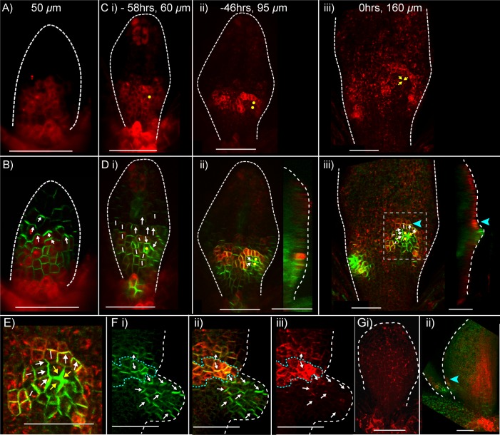
The development of outgrowths from plant shoots depends on formation of epidermal sites of cell polarity convergence with high intracellular auxin at their centre. A parsimonious model for generation of convergence sites is that cell polarity for the auxin transporter PIN1 orients up auxin gradients, as this spontaneously generates convergent alignments. Here we test predictions of this and other models for the patterns of auxin biosynthesis and import. Live imaging of outgrowths from kanadi1 kanadi2 Arabidopsis mutant leaves shows that they arise by formation of PIN1 convergence sites within a proximodistal polarity field. PIN1 polarities are oriented away from regions of high auxin biosynthesis enzyme expression, and towards regions of high auxin importer expression. Both expression patterns are required for normal outgrowth emergence, and may form part of a common module underlying shoot outgrowths. These findings are more consistent with models that spontaneously generate tandem rather than convergent alignments.

Keywords: A. thaliana; CUC; auxin; developmental biology; leaf development; plant biology; polarity; stem cells.

Figure 1.. PIN1::PIN1:GFP expression in young WT and kan1kan2 leaf primordia.

(A) WT primordium of leaf 1, showing abaxial epidermis (a total of 10 leaves were imaged over 2 separate experiments). (B) As for A, but for a kan1kan2 primordium (a total of 15 leaves were imaged over three separate experiments). White arrows indicate inferred polarities. Dashed white lines indicate leaf outlines. Scale bars = 20 µm. DOI: http://dx.doi.org/10.7554/eLife.18165.003

Figure 2.. PIN1::PIN1:GFP polarity patterns in WT and kan1kan2 leaf development.

Confocal images of the PIN1::PIN1:GFP marker in the abaxial epidermis of the same WT leaf primordium imaged over a period of 2 days. Approximate leaf widths (measured from projections of the z stacks) are given above each image. Times from the beginning of the experiment are: i) 0 hrs, ii) 12 hrs, iii) 36 hrs, iv) 48 hrs. Cells indicated by white dots in iii) retain detectable expression of the marker for longer than other cells. This time-lapse data is supported by snapshot images taken for at least five leaves at each developmental stage in a separate experiment. (B) Confocal images of the PIN1::PIN1:GFP marker in the abaxial epidermis of a kan1kan2 leaf primordium, prior to and during the emergence of an ectopic outgrowth. For each time point, a surface view of the abaxial epidermis (left) and a side view of a 3D rendering of the confocal z-stack (right) are shown. The side views allow the emergence of the outgrowth to be monitored. The time relative to when an outgrowth could clearly be observed and the estimated leaf width are given above each image. Yellow arrows in iv) indicate an ectopic centre of PIN1 polarity convergence at the tip of an emerging outgrowth. (C) Magnified images of the regions outlined by the dashed grey rectangles in B, showing the development of the centre of PIN1 polarity convergence at the tip of the emerging outgrowth. Yellow dots, arrows and lines indicate the cells that form the centre of convergence in iv). Arrows indicate inferred PIN1 polarities and lines indicate inferred axes of PIN1 distributions. Scale bars = 20 µm. The scale bar in C i) applies to all panels in C. This data is representative of tracking three out of three kan1kan2 leaves that developed ectopic outgrowths, each in a separate experiment, and with snapshot images from at least three leaves at each developmental stage (in another separate experiment). DOI: http://dx.doi.org/10.7554/eLife.18165.004

Figure 3.. DR5::GFP expression in a kan1kan2 leaf during outgrowth development.

Confocal images of DR5::GFP in the same kan1kan2 leaf imaged over a period of 3 days. Times relative to the first observation of an outgrowth, and leaf widths, are given above images. B ii, C ii and D ii show optical sections through 3D renderings of confocal z-stacks. DR5::GFP (green) and auto-fluorescence plus CUC2::RFP (red) channels are shown (CUC2::RFP is used to help show the leaf outline). Yellow arrows in D indicate the region of DR5::GFP activity at the tip of an outgrowth and yellow arrows in B and C indicate the same DR5::GFP expressing cells tracked back in time prior to outgrowth emergence. White arrow heads indicate high DR5::GFP signal in stipules. Scale bars = 50 µm. This data is representative of tracking 4 out of 4 kan1kan2 leaves that developed outgrowths (in two experiments), and of snapshot data taken for at least 3 leaves at each of the developmental stages shown (in another separate experiment). DOI: http://dx.doi.org/10.7554/eLife.18165.005

Figure 4.. Leaf phenotype of the kan1kan2cuc2 mutant.

(A) Whole kan1kan2 plant. (B) OPT images of a kan1kan2 leaf showing abaxial leaf surface. (C) Whole kan1kan2cuc2 plant. (D) OPT images of a kan1kan2cuc2 leaf. Scale bars in A and C = 1 cm, scale bars in B and D = 1 mm. See Figure 4—figure supplement 1 for more details of the kan1kan2cuc2 phenotype. DOI: http://dx.doi.org/10.7554/eLife.18165.006

Figure 4—figure supplement 1.. Abaxial ridges and serrations produced in kan1kan2cuc2 mutants.

(A) Example of a kan1kan2cuc2 leaf with an abaxial ridge-like thickening (indicated by blue arrow). (B) Example of a kan1kan2cuc2 leaf with serrations. Scale bars = 1 mm. DOI: http://dx.doi.org/10.7554/eLife.18165.007

Figure 5.. PIN1::PIN1:GFP in leaf one of the kan1kan2cuc2 mutant.

(A) Confocal image of PIN1::PIN1:GFP in the abaxial epidermis of the first leaf primordium of a kan1kan2cuc2 mutant. (B) Time-lapse confocal images of the abaxial side of the first leaf of a kan1kan2cuc2 mutant, taken at successive time points. Bi, ii and iii are maximum intensity projections of the abaxial side of the leaf, and therefore signal from both epidermal and sub-epidermal cell layers is combined. The data set shown here is representative of that obtained by tracking three kan1kan2cuc2PIN1::PIN1:GFP leaves (from three different seedlings), and of snapshot images of 10 kan1kan2cuc2 first leaf primordia taken at each of the developmental stages shown. (C) Maximum intensity projection of the abaxial side of leaf 5 of a kan1kan2cuc2 mutant, showing an example of epidermal centres of PIN1 convergence (on left and right sides of the leaf). Scale bars = 50 μm. DOI: http://dx.doi.org/10.7554/eLife.18165.008

Figure 6.. Expression of CUC2::RFPer and PIN1::PIN1:GFP during kan1kan2 outgrowth development.

(A) Confocal images of a CUC2::RFPer reporter in the abaxial epidermis of a young kan1kan2 first leaf primordium. (B) Combined CUC2::RFPer (red) and PIN1::PIN1:GFP confocal channels for the same leaf as in A. White arrows indicate inferred polarity orientations. (C) and (D) Time-lapse imaging of CUC2::RFP and PIN1::PIN1:GFP in the abaxial epidermis of the first leaf of another seedling from that in A and B, over 58 hr prior to outgrowth development. C: CUC2::RFPer, D: combined channels, as in B. Times relative to outgrowth emergence and approximate leaf widths are given above each image. The right-hand images in D ii and iii show optical sections through 3D renderings of the confocal z-stacks at the position of the centre of convergence. White and yellow arrows indicate inferred PIN1 polarity orientations. Yellow dots and arrows indicate the cells that gave rise to the outgrowth tip in C iii and D iii. Blue arrow heads in D iii indicate elevated CUC2::RFPer expression distal to a centre of PIN1 convergence and at the base of the emerging outgrowth on its distal side. Data is representative of that obtained by tracking outgrowth development in five kan1kan2 CUC2::RFPEer PIN1::PIN1:GFP leaves, in three separate experiments. (E) Zoomed-in image of the region outlined by the dashed rectangle in D iii, showing PIN1 polarities within and surrounding the domain of elevated CUC2::RFPer expression. (F) Confocal images of CUC2::RFPer (red) and PIN1::PIN1:GFP (green) associated with an ectopic kan1kan2 outgrowth at a later stage of development to that in C–E. Dotted blue line outlines the domain with elevated CUC2::RFPer expression at the distal boundary between an outgrowth and the main lamina. (G) CUC2::RFPer expression in two WT first leaf primordia (ii also shows PIN::PIN1:GFP in green). Blue arrow in ii indicates a site of elevated CUC2::RFPer expression in the leaf margin. Red signal in the centre of the lamina in ii) is non-ER localised and therefore due to auto-fluorescence. Data is representative of of that obtained by imaging nine leaves at each of the developmental stages shown, across two separate experiments. Scale bars = 50 μm. Dashed white lines indicate leaf outlines. DOI: http://dx.doi.org/10.7554/eLife.18165.009

Figure 7.. Comparison of basic behaviours of indirect coupling, flux-based and up-the-gradient models.

(A–C) Investigating the ability of cells to polarise in the absence of pre-established external asymmetries or polarisable neighbours for up-the-gradient (A), flux-based (B) and indirect coupling (C) models. Panels i) show the initial state of the simulations. In each simulation, all cells initially have the same auxin concentration (indicated by the intensity of green, where darker green indicates a higher concentration). In the case of up-the-gradient or flux-based models (A, B), noise is present in the initial levels of PIN1 (shown by red lines at cell edges). In the case of indirect coupling (C), a single central cell has noise in the levels of A* and B*. Panels ii) show intermediate states of the simulations, and panels iii) show the final states. In this and subsequent simulations, PIN1 polarisation is indicated by black arrows, where the arrow points towards the region of the cell with highest PIN1. (A) For the up-the-gradient model, if a given cell edge has slightly elevated PIN, this causes the juxtaposed neighbour to have an increased auxin concentration. This increased auxin concentration in the neighbour feeds-back to cause increased PIN1 recruitment to the given cell edge (purple arrow in ii). (B) For the flux-based model, a cell edge with a slightly elevated PIN1 concentration causes an increased auxin efflux rate. This increased auxin efflux feeds-back to cause an increased recruitment of PIN1 to the given cell edge (purple arrow in ii). (C) For the indirect coupling model, polarity is generated independently from PIN1 and auxin through A* and B* polarity components (purple arrow in ii) which in turn causes polarisation of PIN1. (D–F) Behaviour of up-the-gradient (D), flux-based (E) and indirect coupling (F) models for 2D arrays of polarisable cells in the absence of pre-established asymmetries. D and E were initialised with noise in the initial concentrations of auxin and F was initialised with noise in the levels A* and B* in the membrane. Details of all simulations can be found in the Materials and methods. See Figure 7—figure supplement 1 for a further comparison of the requirements for polarisation. DOI: http://dx.doi.org/10.7554/eLife.18165.010

Figure 7—figure supplement 1.. Comparison of models’ ability to generate polarity for a cell surrounded by a fixed environment.

In each case the central cell is initialized with noise in the concentrations of PIN at each cell edge and all seven cells have the same auxin concentration. The auxin concentration in each outside neighbor of the central cell is fixed throughout the simulation so that the central cell cannot induce asymmetries in its environment. DOI: http://dx.doi.org/10.7554/eLife.18165.011

Figure 8.. Formation of a proximo-distal polarity field and centres of convergence in the convergent alignment model.

(A) Formation of a proximo-distal polarity field due to the presence of an elevated initial auxin concentration at the leaf tip (orange cells) and an elevated rate of auxin removal from the leaf base (blue cells). The graph shows the concentration of intracellular auxin for each cell in the column marked with the grey arrow. (B) As for A, but for a larger tissue. A centre of polarity convergence forms within the proximal half of the lamina. DOI: http://dx.doi.org/10.7554/eLife.18165.012

Figure 9.. Formation of a proximo-distal polarity field in the flux-based and indirect coupling models.

(A) Formation of a proximo-distal polarity field in the flux-based model due to the presence of elevated auxin biosynthesis at the leaf base (orange cells) and an elevated rate of auxin removal from the leaf tip (blue cells). The graph on the right shows the concentration of intracellular auxin for the column marked with the grey arrow. (B) As for A, but with elevated auxin import (green cell outlines) at the distal end of the tissue. (C) As for A, but for the indirect coupling model. (D) As for B, but for the indirect coupling model. DOI: http://dx.doi.org/10.7554/eLife.18165.013

Figure 10.. Formation of centres of polarity convergence in the flux-based and indirect coupling models.

(A) A proximo-distal polarity field is initially established with the flux based model due to the presence of elevated auxin biosynthesis in the proximal half of the leaf (orange cells) and elevated rates of auxin import and removal from the leaf tip (blue cells with green outlines). The graph on the right shows the concentration of intracellular auxin for the column marked with the grey arrow. Note that there is a broad peak of intracellular auxin concentration within the proximal domain of elevated auxin synthesis (black arrow). (B) Subsequent stage of the simulation in A. If it is assumed that intracellular auxin above a threshold concentration induces elevated auxin import and removal, one or more cells within the proximal domain of elevated auxin biosynthesis are induced to have elevated levels of import and removal. Neighbouring cells reorient their polarity to point towards the high import cells, which accumulate elevated levels of intracellular auxin. (C) As for A), but for the indirect coupling model. (D) As for B), but for the indirect coupling model. See Figure 10—figure supplement 1 for an alternative version of the indirect coupling model which incorporates D6-kinase like activity. DOI: http://dx.doi.org/10.7554/eLife.18165.014

Figure 10—figure supplement 1.. Incorporation of a D6 protein kinase-like activity into the indirect coupling model.

D6 kinase activity was added into simulations of proximodistal polarity establishment (A), (compare with Figure 9D) and convergence formation (B) (compare with Figure 10D). We assume that D6 protein kinase localizes to the A* end of the cell and locally enhances the export of auxin by PIN1. Since A* determines the distribution of PIN1 in the simple form of the indirect coupling model, this addition of D6-kinase-regulated PIN1 activity where A* is present makes little difference to the model’s behaviour. DOI: http://dx.doi.org/10.7554/eLife.18165.015

Figure 11.. Expression of LAX1::GUS and AUX1::AUX1:YFP in WT and kan1kan2 leaves.

(A) Expression pattern of LAX1::GUS in WT leaves one and two. LAX1::GUS was expressed at the tips of developing primordia (arrows in (i), black dashed lines indicate leaf outlines, arrow heads indicate stipules) (a total of 6 plants (with 12 young leaves) were imaged across two separate experiments) and at the tips of serrations (ii) (arrows indicate serrations) (a total of 9 plants (18 leaves) were imaged across three separate experiments). Leaf widths are given above images. (B) Expression pattern of LAX1::GUS in kan1kan2 leaves. LAX1::GUS was expressed at the tips of primordia (i) (a total of 7 plants (14 leaves) were imaged across two separate experiments) and at the tips of outgrowths (ii and iii) (arrows) (20 out of 21 leaves imaged across three separate experiments). ii) shows leaf 1, iii) shows leaf 3. (C) Transverse sections through GUS stained kan1kan2 LAX1::GUS seedlings, showing points of LAX1::GUS expression before outgrowths have emerged (black arrows in i) (data supported by serial sections of 3 other leaves at similar developmental stages in a separate experiment) and at the tips of developing outgrowths (ii) (a total of 8 leaves were imaged across two separate experiments). Dashed orange line in i) indicates leaf outline. (D) AUX1::AUX1:YFP expression in leaf 1 of WT, showing abaxial surface (i) (a total of 15 leaves were imaged across two separate experiments) and adaxial surface (ii) (a total of 4 leaves were imaged in two separate experiments) of two different leaves. (E) AUX1::AUX1:YFP expression in leaf 1 of a kan1kan2 mutant, showing abaxial surface. Arrow points to the tip of an emerging outgrowth with locally elevated AUX1::AUX1:YFP signal (a total of 9 leaves were imaged, across three different experiments). (F) Time-lapse confocal imaging of AUX1::AUX1:YFP in the abaxial epidermis of the first leaf of a kan1kan2 seedling. White arrows mark the positions of cells that eventually gave rise to the AUX1::AUX1:YFP expressing cells in the developing serration on the right side of the leaf. Yellow arrows mark the positions of cells which eventually gave rise to the tip of the ectopic outgrowth on the left side of the leaf. Red and green images in iv), v) and vi) show side views, from the left hand side of the leaf (showing that the outgrowth emerged at the time point shown in v). Red shows auto-fluorescence and a CUC2::RFP marker (used to show the leaf contours), and green shows AUX1::AUX1:YFP signal. Times from the beginning of the experiment at which images were taken are: i) 0 hrs, ii) 22 hr 40 min, iii) 31 hr 10 min, iv) 46 hr 40 min, v) 55 hr 40 min, vi) 74 hr 40 min. Data is consistent with tracking experiments performed for two other kan1kan2 leaves that developed ectopic outgrowths, and with snapshot images of at least 6 leaves before and after outgrowth emergence. (G) Mean number of outgrowths (+/- standard error of the mean) in rosette leaves of kan1kan2 plants carrying mutant alleles of AUX/LAX genes. n numbers are: kan1kan2: 84 leaves from 10 plants, kan1kan2aux1lax1: 110 leaves from 10 plants, kan1kan2aux1lax1lax2: 136 leaves from 10 plants, kan1kan2aux1lax1lax2lax3:200 leaves from 10 plants. (H) Convergent alignment model where elevated intracellular auxin causes elevated rates of auxin import and removal. The model is initialised with elevated auxin degradation at the leaf base (blue cells) and an elevated rate of auxin import and degradation at the leaf tip (blue cells with green outlines). Centres of convergence form within the proximal half of the lamina and when the intracellular auxin concentration exceeds a threshold level, an elevated rate of auxin import and removal is induced (blue cells with green outlines). Scale bars = 50 µm. See Figure 11—figure supplement 1 for LAX2::GUS and LAX3::GUS expression. DOI: http://dx.doi.org/10.7554/eLife.18165.016

Figure 11—figure supplement 1.. Expression patterns of LAX2::GUS and LAX3::GUS.

(A) Expression of LAX2::GUS in a kan1kan2+/- leaf, showing expression in leaf vascular tissue. Scale bar = 100 μm. (B) Expression of LAX3::GUS in a WT seedling, showing expression is absent from leaves, but present in the hypocotyl and root. Scale bar = 1 mm (C) Expression of LAX3::GUS in a kan1kan2 seedling. Scale bars = 100 μm. DOI: http://dx.doi.org/10.7554/eLife.18165.018

Figure 12.. LAX1 and AUX1 expression in kan1kan2cuc2 mutants.

(A) Expression of LAX1::GUS in the abaxial surface of leaf 1 of a kan1kan2cuc2 mutant. Data representative of images from ten seedlings in two separate experiments. (B) AUX1::AUX1:YFP expression in leaf 3 and 4 of a kan1kan2cuc2 mutant. Images representative of those taken from fifteen seedlings in two separate experiments. (C) CUC2::RFPer and AUX1::AUX1:YFP expression in leaf 3 of a kan1kan2 mutant leaf i) AUX1::AUX1:YFP, ii) CUC2::RFPer (red) and AUX1::AUX1:YFP (green), iii) CUC2::RFPer. White arrows indicate region of low AUX1::AUX1:YFP and elevated CUC2::RFPer expression at the distal base of developing outgrowths. Images representative of those taken from six seedlings in two experiments. Approximate leaf widths are given above each image. Scale bars = 50 μm. DOI: http://dx.doi.org/10.7554/eLife.18165.019

Figure 13.. PIN1 immuno-localisation in transverse cross-sections of kan1kan2 leaves.

(A) PIN1 immuno-localisation in a kan1kan2 leaf before outgrowth emergence. i) and ii) are consecutive sections through the tissue (each section is 8 µm thick). A centre of PIN1 polarity convergence can be seen in i) and the site of this convergence is shown with yellow arrows in ii). Arrows show the inferred directions of PIN1 polarity. The adaxial side of the leaf is at the top of the image. 4 leaves with convergences were imaged across two separate experiments. (B) PIN1 immuno-localisation in a kan1kan2 leaf in which outgrowths have begun to emerge. Dotted white lines indicate the strands of cells with elevated levels of PIN1 and the leaf outline. 3 leaves with emerging outgrowths were imaged across two separate experiments. All scale bars = 50 μm, except those in the zoomed in panels in A, which are 10 μm. DOI: http://dx.doi.org/10.7554/eLife.18165.020

Figure 14.. YUCCA1::GUS expression in WT leaves.

(A) Expression of YUC1::GUS in a WT leaf 1 primordium. i) abaxial epidermis (10 plants were imaged across two separate experiments) ii) transverse cross-sectional view of leaf 1 at a similar developmental stage (adaxial (ad) is towards the top) at the position marked by the dashed black line in i). Dashed orange line indicates leaf outline. Data consistent with serial sections taken through 3 other leaves. (B) Transverse cross-sectional view of a YUC1::GUS expressing wild-type vegetative meristem. Yellow arrow with black outline indicates region of YUC1::GUS expression at the boundary of an emerging primordium. Dashed orange lines indicate leaf primordia outlines. Data consistent with sections from 3 meristems, across two separate experiments. (C) Expression of YUC1::GUS at a later stage of WT leaf development. Scale bars = 50 µm. 9 leaves imaged across two separate experiments. (D) In the presence of elevated auxin production in the proximal row of cells (orange), and elevated auxin import and removal in the distal row of cells (blue cells with green outline), the convergent alignment model generates a divergent polarity field, with proximally oriented polarity in the proximal half of the tissue, and distally oriented polarity in the distal half. DOI: http://dx.doi.org/10.7554/eLife.18165.021

Figure 15.. Expression of YUCCA1::GUS in kan1kan2 leaves.

(A) Expression of YUC1::GUS in kan1kan2 leaf one primordia. i) abaxial epidermis (a total of 15 leaves imaged, in three separate experiments), ii) transverse cross-sectional view of leaf 1 at a similar developmental stage, at an approximate position along the proximo-distal axis marked with the pink dashed line in i, iii) transverse cross section through the same leaf as shown in ii), at the approximate position marked with the green dashed line in i. Data consistent with serial sections for 3 other kan1kan2 leaves. (B) Expression of YUC1::GUS in kan1kan2 mutant leaf 1 primordia at progressive stages of development. Black arrows indicate the band of YUC1::GUS expression, which is at the distal base of outgrowths in iii) and iv). Arrow heads indicate an outgrowth tip which does not express YUC1::GUS. At least 8 leaves were imaged for each developmental stage, across two experiments. (C) Expression of LAX1::GUS in first two leaves of a kan1kan2yuc1yuc4 seedling (a total of 20 leaves were imaged in three separate experiments). (D) Expression of YUC1::GUS in leaf one of kan1kan2cuc2 mutant seedlings (15 seedlings were imaged at each developmental stage across three separate experiments). Scale bars = 50 µm. DOI: http://dx.doi.org/10.7554/eLife.18165.022

Figure 16.. Effect of a band of locally elevated auxin biosynthesis on flux-based, indirect coupling and up-the-gradient models.

(A) Flux-based model. A proximodistal polarity field is initially established due to elevated auxin production at the leaf base (orange cells) and elevated auxin import and removal at the leaf tip (blue cells with green outline). After distally oriented polarities are established, 3 cells are given an elevated rate of auxin biosynthesis (orange cells), causing polarities to diverge away from this region. Graph shows intracellular auxin concentrations for the column of cells marked with the grey arrow. (B) As for A, but with a cell with elevated auxin import and removal (blue cell with green outline) on the proximal side of the band with elevated auxin synthesis. (C) As for A, but for the indirect coupling model. (D) As for B, but for the indirect coupling model. (E) Up the gradient model. A proximo-distal polarity field is initially established through elevated auxin removal at the leaf base (blue cells) and an initially elevated auxin concentration at the leaf tip (same initial conditions as Figure 8A). Three cells (isolated orange cells) are then given an elevated auxin biosynthesis rate, causing polarities to orient towards them. (F) As for E, but a cell with elevated auxin import and removal is also added on the proximal side of the band with elevated auxin synthesis. DOI: http://dx.doi.org/10.7554/eLife.18165.023

Figure 17.. Time-lapse imaging of YUC4::GFP in kan1kan2 leaves.

(A) Confocal images of YUC4::GFP in the same kan1kan2 leaf imaged over a period of 3 days. Times relative to outgrowth emergence, and leaf widths, are given above images. Yellow circles indicate cells located distal to the outgrowth after its emergence, and their ancestors prior to outgrowth emergence. Note that these cells express YUC4::GFP before and after outgrowth emergence, but the region of expression at the outgrowth tip only appears following outgrowth emergence. Data is representative of tracking 5 out of 5 kan1kan2 leaves that developed ectopic outgrowths across two experiments. (B) YUC4::GFP expression in leaf one of a kan1kan2cuc2 mutant. Data representative of 13 leaves imaged in two separate experiments. Arrow head indicates stipule. Scale bars = 50 µm. DOI: http://dx.doi.org/10.7554/eLife.18165.024

Figure 18.. Classification of plant and animal polarity models.

Models of plant and animal epidermal polarity may be classified according to whether they require the presence of pre-established asymmetries or polarisable neighbours (referred to as a polarising environment) for cell polarity to arise. All plant models tested can generate cell polarity without a polarising environment, whilst animal models except the direct coupling model ([4] [Abley et al., 2013]) either require an asymmetric signal ([1] [Le Garrec et al., 2006] [2] [Amonlirdviman, 2005]) or polarisable neighbours ([3] [Burak and Shraiman, 2009]) for cell polarity to arise. A further classification is made according to the behaviours of groups of cells in the absence of pre-established asymmetries. In this context, the indirect coupling ([5] [Abley et al., 2013]) and flux-based ([6] [Mitchison, 1980; Rolland-Lagan and Prusinkiewicz, 2005; Stoma et al., 2008]) models of plant polarity generate swirled patterns of polarity with tandem alignments between cells. In contrast, the up-the-gradient model ([7] [Bilsborough et al., 2011; Jönsson et al., 2006; Smith et al., 2006]) generates convergent alignments of cell polarities. The stress-based model of PIN1 polarity ([8] [Heisler et al., 2010]) also fits in the convergent alignment category as it generates similar behaviours with respect to auxin concentrations to the up-the-gradient model. The animal models that are capable of polarising in the absence of pre-established asymmetries generate tandem alignments of polarities ([4] direct coupling model [Abley et al., 2013], and (3) Burak and Shraiman, 2009). DOI: http://dx.doi.org/10.7554/eLife.18165.025

References

1. Abley K, De Reuille PB, Strutt D, Bangham A, Prusinkiewicz P, Maree AFM, Grieneisen VA, Coen E. An intracellular partitioning-based framework for tissue cell polarity in plants and animals. Development. 2013;140:2061–2074. doi: 10.1242/dev.062984. - DOI - PubMed
1. Aida M, Ishida T, Fukaki H, Fujisawa H, Tasaka M. Genes involved in organ separation in arabidopsis: An analysis of the cup-shaped cotyledon mutant. The Plant Cell Online. 1997;9:841–857. doi: 10.1105/tpc.9.6.841. - DOI - PMC - PubMed
1. Amonlirdviman K, Khare NA, Tree DR, Chen WS, Axelrod JD, Tomlin CJ. Mathematical modeling of planar cell polarity to understand domineering nonautonomy. Science. 2005;307:423–426. doi: 10.1126/science.1105471. - DOI - PubMed
1. Bainbridge K, Guyomarc'h S, Bayer E, Swarup R, Bennett M, Mandel T, Kuhlemeier C. Auxin influx carriers stabilize phyllotactic patterning. Genes & Development. 2008;22:810–823. doi: 10.1101/gad.462608. - DOI - PMC - PubMed
1. Barbosa IC, Zourelidou M, Willige BC, Weller B, Schwechheimer C. D6 PROTEIN KINASE activates auxin transport-dependent growth and PIN-FORMED phosphorylation at the plasma membrane. Developmental Cell. 2014;29:674–685. doi: 10.1016/j.devcel.2014.05.006. - DOI - PubMed
Publication types