Spatially-explicit models of global tree density

Abstract

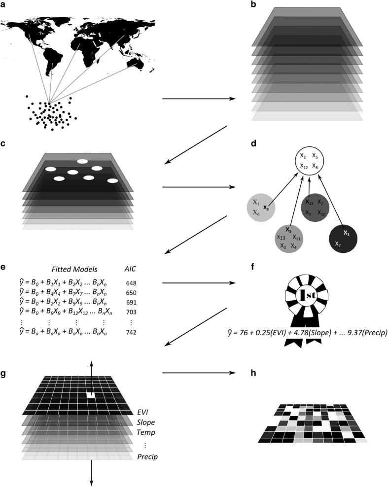
Remote sensing and geographic analysis of woody vegetation provide means of evaluating the distribution of natural resources, patterns of biodiversity and ecosystem structure, and socio-economic drivers of resource utilization. While these methods bring geographic datasets with global coverage into our day-to-day analytic spheres, many of the studies that rely on these strategies do not capitalize on the extensive collection of existing field data. We present the methods and maps associated with the first spatially-explicit models of global tree density, which relied on over 420,000 forest inventory field plots from around the world. This research is the result of a collaborative effort engaging over 20 scientists and institutions, and capitalizes on an array of analytical strategies. Our spatial data products offer precise estimates of the number of trees at global and biome scales, but should not be used for local-level estimation. At larger scales, these datasets can contribute valuable insight into resource management, ecological modelling efforts, and the quantification of ecosystem services.

Figure 1. A conceptual model of our analytical process.

(a) We amassed over 420,000 forest inventory plot records from every continent except Antarctica. (b) We acquired and unified an initial pool of four-dozen spatial covariates to use in model development. (c) We selected a subset of spatial covariates, extracted their values at field plot locations, and bound these values to the plot records. (d) For each of 14 biomes we subjected the enhanced plot records to hierarchical (agglomerative) clustering to identify the least collinear collection of covariates. (e) Generalized linear models were fit to every possible combination of clustered covariates. (f) A top ranking predictive model was selected or created through model averaging. (g) Each biome’s top ranking model was applied in a pixel-level map algebraic framework. (h) We scaled a penultimate spatial model of tree density using land cover data to arrive at our final predictions.

Figure 2. Statistical and spatial model validation.

(a) The standard deviation of the predicted mean number of trees per biome as a function of sample size. As sample size increases, the variability of the predicted mean tree density reaches a threshold, beyond which an increase in sample size results in a minimal increase in precision. Standard deviations were calculated using a bootstrapping approach (see Statistical model validation), and smooth curves were modeled using standard linear regression with a log–log transformation. After Crowther et al (2015) Fig. 3b. (b) Biome-level regression models predict the mean values of the omitted validation plot measurements in 12 biomes. Overall, the models underestimated mean tree density by ~3% (slope=0.97) but this difference was not statistically significant (P=0.51). Bars show±one s.d. for the predicted mean and the dotted boundaries represent the 95% confidence interval for the mean. The values plotted here represent mean densities for the plot measurements (that is, for forested ecosystems), rather than those predicted for each entire biome. Figure is modified from Crowther et al (2015) Fig. 3a.

Figure 3. Global models of tree density.

Tree density as portrayed through biome- (a) and ecoregion-level (b) models where values represent number of trees per ~1 km² pixel. Actual pixel size, 897.27 m by 897.27 m in the Goode Homolosine projection. All computations based on areal measurements were made using Goode Homolosine. Maps were produced using ESRI basemap imagery.

Figure 4. Correlation of predicted and published numbers of trees per country.

The dotted line is a 1:1 line, while the solid line is the ordinary least squares line of best fit. Figure is modified from Crowther et al (2015) Fig. 4d.

References

Data Citations
1. Crowther T. W. 2015. EliScholar. http://elischolar.library.yale.edu/yale_fes_data/1
1. Crowther T. W. 2016. Figshare. http://dx.doi.org/10.6084/m9.figshare.3179986 - DOI
1. Crowther T. W. et al. Mapping tree density at a global scale. Nature 525, 201–205 (2015). - PubMed
1. ter Steege H. et al. Hyperdominance in the Amazonian tree flora. Science 342, 1243092 (2013). - PubMed
1. Nadkarni N. Between Earth and Sky: Our Intimate Connections to Trees (University of California Press, 2008).
1. FAO. Global Forest Resources Assessment 2010 - Main Report. (Rome, Italy (2010).
1. Chisholm R. A. et al. Scale-dependent relationships between tree species richness and ecosystem function in forests. J. Ecol. 101, 1214–1224 (2013).
Publication types