. 2016 Aug 17;36(33):8598-611.
doi: 10.1523/JNEUROSCI.0184-16.2016.

Dynamic Multisensory Integration: Somatosensory Speed Trumps Visual Accuracy during Feedback Control

Affiliations

Dynamic Multisensory Integration: Somatosensory Speed Trumps Visual Accuracy during Feedback Control

Frédéric Crevecoeur et al. J Neurosci. .

Abstract

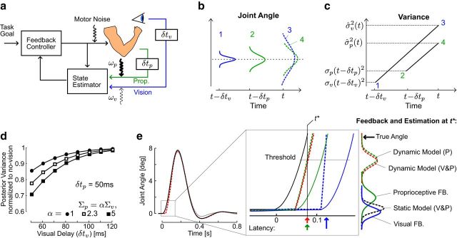
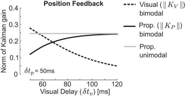
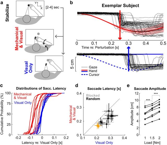
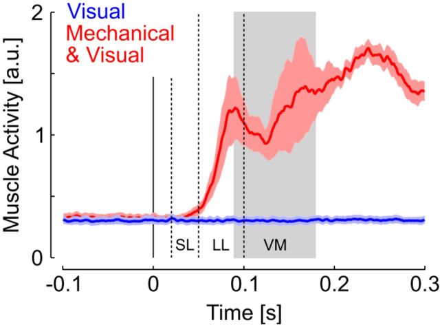
Recent advances in movement neuroscience have consistently highlighted that the nervous system performs sophisticated feedback control over very short time scales (<100 ms for upper limb). These observations raise the important question of how the nervous system processes multiple sources of sensory feedback in such short time intervals, given that temporal delays across sensory systems such as vision and proprioception differ by tens of milliseconds. Here we show that during feedback control, healthy humans use dynamic estimates of hand motion that rely almost exclusively on limb afferent feedback even when visual information about limb motion is available. We demonstrate that such reliance on the fastest sensory signal during movement is compatible with dynamic Bayesian estimation. These results suggest that the nervous system considers not only sensory variances but also temporal delays to perform optimal multisensory integration and feedback control in real-time.

Significance statement: Numerous studies have demonstrated that the nervous system combines redundant sensory signals according to their reliability. Although very powerful, this model does not consider how temporal delays may impact sensory reliability, which is an important issue for feedback control because different sensory systems are affected by different temporal delays. Here we show that the brain considers not only sensory variability but also temporal delays when integrating vision and proprioception following mechanical perturbations applied to the upper limb. Compatible with dynamic Bayesian estimation, our results unravel the importance of proprioception for feedback control as a consequence of the shorter temporal delays associated with this sensory modality.

Keywords: decision making; motor control; multisensory integration; state estimation.


Figures

Figure 1.
Figure 1.
Dynamic Bayesian model. a, Illustration of the real-time feedback controller based on state estimation. The model considers two sources of sensory information (vision, blue; limb afferent feedback, green) affected by distinct temporal delays (δtp.v) and sensory noise (ωp,v). b, Schematic representation of how uncertainty in sensory feedback increase over time. Green and blue distributions correspond to the feedback about limb motion at two distinct points in time, and the dashed distributions show how related estimates in the present state are impacted by the accumulation of uncertainty over the delay period. c, Schematic illustration of how the increase in variance over the delay period can lead to higher uncertainty associated with vision. The variances of proprioceptive and visual signals are σp(t − δtp)2 and σv(t − δtv)2 and the variance of the estimated states at the present time are σ̂p,v2. d, Theoretical posterior variance of the joint angle estimate for distinct values of visual delays and distinct variance ratios. The posterior variance was normalized to the value obtained without visual feedback, so that a value of 1 indicates equal posterior variances with or without vision. The value of 2.3 corresponds to weighting vision by 70% and proprioception by 30%. e, Changes in actual (solid) or estimated (dashed) angle following a step torque applied on the joint. Solid traces represent simulated perturbations with (black) or without (gray) vision. The two traces are superimposed for almost the entire course of the corrective response. The inset magnifies the actual angle (solid black), delayed feedback (proprioception in solid green and vision in solid blue), and estimated angles following the perturbation computed by the Kalman filter. Vertical arrows represent hypothetical estimation latency with vision only (blue), proprioception only (green), or combined visual and proprioceptive feedback (red) based on exemplar threshold crossed at t*. Distributions represent the sensory feedback or estimated joint angle at t* (vertical thin line).
Figure 2.
Figure 2.
Norm of Kalman gains. Effect of sensory delays on the norm of the block components of the Kalman gain matrix (Eq. 8). Black traces correspond to situations in which vision (dashed) and proprioception (solid) are available (bimodal). The gray correspond to situations in which proprioception is the only source of sensory feedback available (unimodal). Displays are the norm of the block components of the Kalman gain matrix influencing the estimation of the joint angle. All values were calculated with Σp = 2.3 × Σv as reported in previous work.
Figure 3.
Figure 3.
Results of Experiment 1. a, Experimental paradigm. Participants were instructed to stabilize in the start target (top), then to visually track the cursor (small black dot) following Mechanical and Visual perturbation (red) or Visual Only (blue). The big gray dot illustrates the target used during the postural control task. The curved arrows (middle) illustrate the multi-joint perturbation torque applied on the limb. b, Individual eye movements from one representative subject (thin black), and average hand movement (solid) or cursor movement (dashed). The shaded area represents 1 SD across trials (hand and cursor traces are superimposed for the Mechanical and Visual perturbations). The vertical arrows illustrate the average saccade latency following combined mechanical and visual perturbations (red, top), or visual only (blue, bottom). c, Individuals' cumulative distributions of saccade latencies aligned on the 50th percentile of the distribution of responses to visual perturbations for each subject. d, Saccade latencies following each perturbation type. Crosses represent the mean ± SD across trials for each individual subject. Black and gray crosses correspond to random and blocked conditions, respectively. The orange crosses represent data from participants tracking a physical LED without any virtual reality display (see Materials and Methods, Control experiments). e, Modulation of saccade amplitude across perturbation magnitudes. Connected dots are the average saccade amplitude as a function of the perturbation load for each participant. Stars indicate significant differences based on paired comparisons with post hoc Bonferroni corrections (see Materials and Methods).
Figure 4.
Figure 4.
Muscle responses to mechanical perturbations. Grand average of muscle activity across muscle samples and participants. Traces were smoothed with a 10 ms moving average for illustration purposes. Colored areas represent 1 SE across participants. The vertical dashed lines delineate the epochs of motor responses (SL: 20–50 ms; LL: 50–100 ms), and the gray rectangle corresponds to the time window associated with rapid visuomotor feedback (90–180 ms).
Figure 5.
Figure 5.
Smooth eye displacement. a, Gaze velocity following the onset of the mechanical (red) or visual (blue) perturbations. The gray rectangle illustrates the time window of 70–120 ms, during which the gaze velocity following mechanical perturbations displayed significant modulation toward the fingertip. b, Gaze displacement toward the target. Traces were aligned on saccade onset. a, b, Shaded areas represent SE across participants.
Figure 6.
Figure 6.
Results of Experiment 2. a, Illustration of the three perturbation types: Mechanical Only (green, M) during which the hand aligned cursor was extinguished, Mechanical and Visual (M and V, red), and Visual Only (V). The initial stabilization was identical to the first experiment and was omitted here for clarity. Inset, The endpoint error vector computed as the difference between the hand or cursor and gaze coordinates at the end of the first saccade. b, Average (solid) and SD (shaded area) of fingertip or cursor motion from one exemplar subject with similar color codes as in a. The gaze coordinate from individual trials is represented with thin black traces. Colored arrows and vertical dashed lines are aligned on the average SRT for this representative participant with the same color code as in a. Observed that the red arrow is aligned on the average SRT from the purely mechanical condition c, Saccade endpoints from one representative subject relative to the fingertip and/or cursor location. Errors are mainly located in the first quadrant following elbow flexor loads. Two-dimesional ellipses obtained from singular value decomposition of the saccade endpoint distribution are presented for each perturbation following the same color code as in a and b. d, Saccade latency (left), norm of endpoint error (center) and two-dimensional endpoint dispersion computed as the area of the endpoint dispersion ellipses as represented in c. Error bars represent 1 SEM across participants. Significant differences revealed by paired comparisons with post hoc Bonferroni corrections are illustrated with *p < 0.05 or **p < 0.01.
Figure 7.
Figure 7.
Results of the second control experiment. a, Illustration of the three perturbation types used in this control experiment. For Mechanical Perturbations only (M), the hand-aligned cursor (black dot) remained attached to the target. These mechanical perturbation trials are illustrated in black to emphasize that they are distinct from the purely mechanical perturbations used in Experiment 2. Visual (V, blue) and combined Mechanical and Visual perturbations (M and V, red) were identical to those of Experiment 2. The initial stabilization was identical to the first experiment and was omitted here for clarity. b, Saccadic reaction times across blocks with similar color code as in Figure 6a. Significant differences from paired comparisons at the level are represented with *p < 0.05 and **p < 0.01. c, Norm of the saccade endpoint error (left) and endpoint variance measured as the area of the two-dimensional dispersion ellipses as in Figure 6. Vertical bars represent the SEM across participants.
Figure 8.
Figure 8.
Relationship between SRT and accuracy. a, Relationship between saccade latency and endpoint error from one representative subject (data from Experiment 2). Ellipses represent the 1 SD along each axis. Dots represent individual trials. b, Left, Polar plot representing the ellipses computed from each participant. The radii are the ellipses aspect ratio (ie, the ratio between principal and secondary components), and the angles represent the orientation of the principal component (PC) mapped between −90° and 90°. The norm of error and latency were expressed in meters and seconds before computing the ellipses orientation and aspect ratios, such that an angle of 45° corresponds to a slope of 1 (observe that the axes in a have different scales for illustration). Right, Comparison of principal component angle and of the aspect ratio across the three perturbation types. Significant differences are illustrated (paired comparisons, p < 0.01).
Figure 9.
Figure 9.
Upper-limb motor corrections. a, Ensemble average of perturbation-related changes in shoulder (dashed) and elbow (solid) joints following positive (flexion) perturbations. Perturbation trials with or without visual feedback are represented in red or green, respectively (data from Experiment 3). Thin lines represent 1 SEM. The vertical arrows illustrate the estimated time when vision contributes to reducing the endpoint variability (black arrow), as well as the movement end estimated from hand velocity (gray arrow; see Materials and Methods). b, Top, Two-dimensional fingertip dispersion area following perturbations (mean ± SEM). The SD area was computed from the covariance matrix of x- and y-coordinates at each time step. The area of fingertip dispersion across trials was computed for each perturbation direction independently, and averaged across directions (see Materials and Methods). Bottom, Time series of p values from paired t test comparison of fingertip standard dispersion across conditions with or without visual feedback. The black arrows corresponds to the time when the p value becomes <0.05.

Similar articles

Cited by

References

    1. Anderson BDO, Moore JD. Optimal filtering. Engelwood Cliffs, New Jersey: Prentice-Hall; 1979.
    1. Angelaki DE, Gu Y, DeAngelis GC. Multisensory integration: psychophysics, neurophysiology, and computation. Curr Opin Neurobiol. 2009;19:452–458. doi: 10.1016/j.conb.2009.06.008. - DOI - PMC - PubMed
    1. Ariff G, Donchin O, Nanayakkara T, Shadmehr R. A real-time state predictor in motor control: study of saccadic eye movements during unseen reaching movements. J Neurosci. 2002;22:7721–7729. - PMC - PubMed
    1. Bhushan N, Shadmehr R. Computational nature of human adaptive control during learning of reaching movements in force fields. Biol Cybern. 1999;81:39–60. doi: 10.1007/s004220050543. - DOI - PubMed
    1. Blohm G, Missal M, Lefèvre P. Processing of retinal and extraretinal signals for memory-guided saccades during smooth pursuit. J Neurophysiol. 2005;93:1510–1522. doi: 10.1152/jn.00543.2004. - DOI - PubMed

Publication types

LinkOut - more resources