Mapping transiently formed and sparsely populated conformations on a complex energy landscape

Abstract

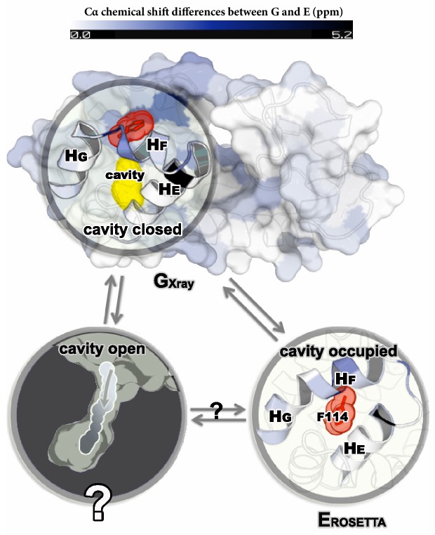
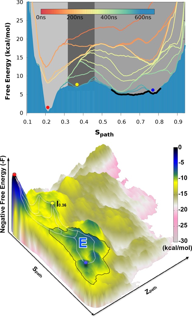
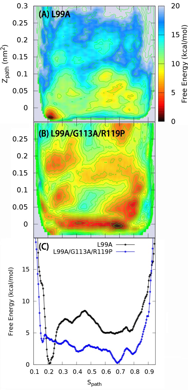
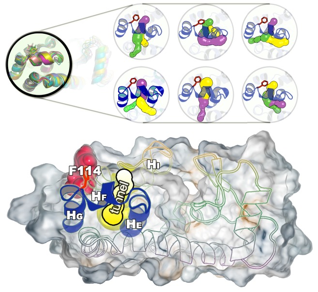
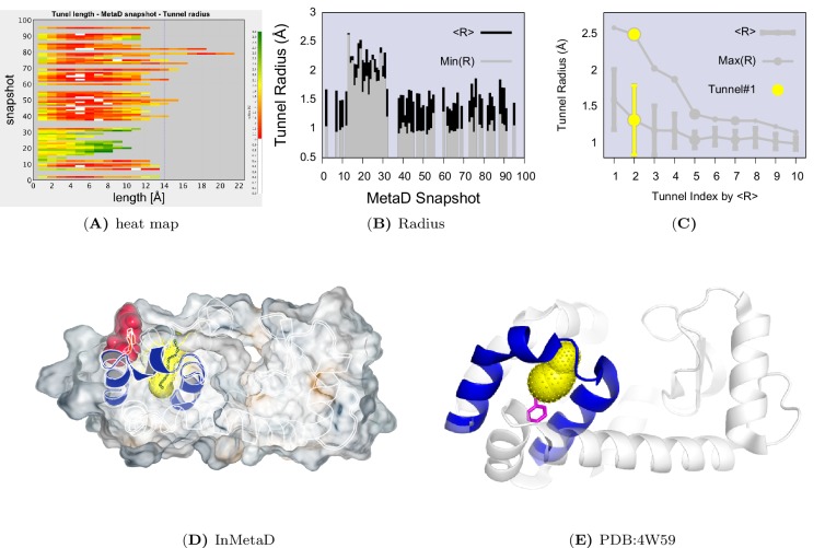
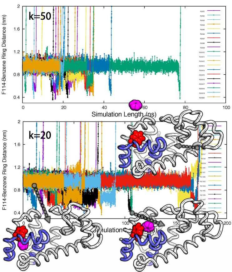
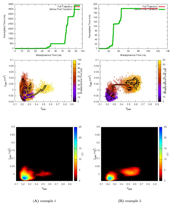
Determining the structures, kinetics, thermodynamics and mechanisms that underlie conformational exchange processes in proteins remains extremely difficult. Only in favourable cases is it possible to provide atomic-level descriptions of sparsely populated and transiently formed alternative conformations. Here we benchmark the ability of enhanced-sampling molecular dynamics simulations to determine the free energy landscape of the L99A cavity mutant of T4 lysozyme. We find that the simulations capture key properties previously measured by NMR relaxation dispersion methods including the structure of a minor conformation, the kinetics and thermodynamics of conformational exchange, and the effect of mutations. We discover a new tunnel that involves the transient exposure towards the solvent of an internal cavity, and show it to be relevant for ligand escape. Together, our results provide a comprehensive view of the structural landscape of a protein, and point forward to studies of conformational exchange in systems that are less characterized experimentally.

Keywords: biochemistry; biophysics; conformational exchange; free energy landscape; kinetics; molecular dynamics; nuclear magnetic resonance; structural biology.

Figure 1.. Structures of the major G and minor E states of L99A T4L and the hidden state hypothesis.

The X-ray structure of the G state ($G_{Xray}$; PDB ID code 3DMV) has a large internal cavity within the core of the C-terminal domain that is able to bind hydrophobic ligands. The structure of the E state ($E_{ROSETTA}$; PDB ID code 2LC9) was previously determined by CS-ROSETTA using chemical shifts. The G and E states are overall similar, apart from the region surrounding the internal cavity. Comparison of the two structures revealed two remarkable conformational changes from G to E: helix F (denoted as $H_F$) rotates and fuses with helix G ($H_G$) into a longer helix, and the side chain of phenylalanine at position 114 ($F_{114}$) rotates so as to occupy part of the cavity. As the cavity is inaccessible in both the $G_{Xray}$ and $E_{ROSETTA}$ structures it has been hypothesized that ligand entry occurs via a third ‘cavity open’ state (Merski et al., 2015). DOI: http://dx.doi.org/10.7554/eLife.17505.003

Figure 2.. Free energy landscape of the L99A variant of T4L.

In the upper panel, we show the projection of the free energy along $S_{path}$, representing the Boltzmann distribution of the force field employed along the reference path. Differently colored lines represent the free energy profiles obtained at different stages of the simulation, whose total length was 667ns. As the simulation progressed, we rapidly found two distinct free energy basins, and the free energy profile was essentially constant during the last 100 ns of the simulation. Free energy basins around $S_{path}=0.2$ and $S_{path}=0.75$ correspond to the previously determined structures of the G- and E-state, respectively (labelled by red and blue dots, respectively). As discussed further below, the E-state is relatively broad and is here indicated by the thick, dark line with $S_{path}$ ranging from 0.55 to 0.83. In the lower panel, we show the three-dimensional negative free energy landscape, -F($S_{path}$, $Z_{path}$), that reveals a more complex and rough landscape with multiple free energy minima, corresponding to mountains in the negative free energy landscape. An intermediate-state basin around $S_{path}=0.36$ and ${\displaystyle Z_{path}=0.05}$ nm², which we denote $I_{0.36}$, is labeled by a yellow dot. DOI: http://dx.doi.org/10.7554/eLife.17505.004

Figure 2—figure supplement 1.. Approximately equidistant frames along the reference path.

The plot reveals a ‘gullwing’ shape of the matrix of pairwise RMSDs of the frames of the reference path, indicating that frames along the reference path are approximately equidistant. We used 31 structures to discretize the path. DOI: http://dx.doi.org/10.7554/eLife.17505.005

Figure 2—figure supplement 2.. One and two dimensional free energy landscape of L99A and the triple mutant.

(A) The two-dimensional free energy surface F($S_{path}$,$Z_{path}$) of L99A sampled by a 667 ns PathMetaD simulation. (B) The two-dimensional free energy surface F($S_{path}$,$Z_{path}$) of the triple mutant sampled by a 961 ns PathMetaD simulation. (C) The free energy profiles as a function of $S_{path}$ of both L99A (black) and the triple mutant (blue). DOI: http://dx.doi.org/10.7554/eLife.17505.006

Figure 3.. Estimation of free energy differences and comparison with experimental measurements.

We divided the global conformational space into two coarse-grained states by defining the separatrix at $S_{path}=0.46$ (0.48 for the triple mutant) in the free energy profile (Figure 2—figure supplement 2) which corresponds to a saddle point of the free energy surface, and then estimated the free energy differences between the two states ($\mathrm{\Delta }G$) from their populations. The time evolution of $\mathrm{\Delta }G$ of L99A (upper time axis) and the triple mutant (lower axis) are shown as black and blue curves, respectively. The experimentally determined values (2.1 kcal mol⁻¹ for L99A and −1.9 kcal mol⁻¹ for the triple mutant) are shown as yellow lines. DOI: http://dx.doi.org/10.7554/eLife.17505.007

Figure 4.. Conformational ensemble of the minor state as determined by CS biased, replica-averaged simulations.

We determined an ensemble of conformations corresponding to the E-state of L99A T4L using replica-averaged CSs as a bias term in our simulations. The distribution of conformations was projected onto the $S_{path}$ variable (orange) and is compared to the free energy profile obtained above from the metadynamics simulations without experimental biases (black line). To ensure that the similar distribution of conformations is not an artifact of using the same force field (CHARMM22*) in both simulations, we repeated the CS-biased simulations using also the Amber ff99SB*-ILDN force field (magenta) and obtained similar results. Finally, we used the ground state CSs of a triple mutant of T4L, which was designed to sample the minor conformation (of L99A) as its major conformation, and also obtained a similar distribution along the $S_{path}$ variable (cyan). DOI: http://dx.doi.org/10.7554/eLife.17505.009

Figure 4—figure supplement 1.. Equilibrium sampling of conformational regions of the E state of L99A by CS-restrained replica-averaged simulation.

We calculated the RMSD between the experimental CSs and the values back-calculated by CamShift (Kohlhoff et al., 2009) as implemented in ALMOST (Fu et al., 2014). We projected a 250 ns MD trajectory sampled using the CHARMM22* force field (RUN3 in Appendix 1—table 1) onto the RMSDs. The average RMSDs for the five measured nuclei ($H_{\alpha }$, $H_N$, $N$, $C^{\prime }$ and $C_{\alpha }$) are 0.23 ppm, 0.38 ppm, 1.97 ppm, 0.83 ppm and 1.06 ppm, respectively (Appendix 1—table 2), which are close to the inherent uncertainty of the chemical shift calculation (Figure 4—figure supplement 2). This indicates the simulation yielded an ensemble in good agreement with experiments. DOI: http://dx.doi.org/10.7554/eLife.17505.010

Figure 4—figure supplement 2.. Estimation of the inherent uncertainty of the chemical shift calculation by different algorithms: CamShift (Kohlhoff et al., 2009), ShiftX (Neal et al., 2003) and Sparta+ (Shen and Bax, 2010).

Using $E_{ROSETTA}$ as the reference structure, we calculated the chemical shifts using different algorithms and compared the correlation coefficients and RMSD between them. DOI: http://dx.doi.org/10.7554/eLife.17505.011

Figure 4—figure supplement 3.. Force field dependency of the replica averaged MD simulations of L99A with chemical shift restraints.

The chemical shifts of the E state of L99A (BMRB 17604) were used. (A) The simulation with CHARMM22* force field. (B) The simulation with Amber ff99SB*-ILDN force field. DOI: http://dx.doi.org/10.7554/eLife.17505.012

Figure 4—figure supplement 4.. Effect of changing the force constant and number of replicas in CS-restrained simulation of L99A.

(A) N = 4, ${\displaystyle {ϵ}_{CS}=24}$ KJ · mol⁻¹. (B) N = 2, ${\displaystyle {ϵ}_{CS}=24}$ KJ · mol⁻¹. (C) N = 2, ${\displaystyle {ϵ}_{CS}=12}$ KJ · mol⁻¹. N refers to the number of replicas that the CS values are averaged over. The CHARMM22* force field was used in these simulations. The results also support the conclusion that the conformational space of the minor (E) state covers a relatively wide set of structures including the $E_{ROSETTA}$ structure. DOI: http://dx.doi.org/10.7554/eLife.17505.013

Figure 4—figure supplement 5.. Replica-averaged CS-restrained MD simulation of a T4L triple mutant (L99A/G113A/R119P).

Chemical shift restraints were from BMRB 17,603 and CHARMM22* force field was used. DOI: http://dx.doi.org/10.7554/eLife.17505.014

Figure 5.. Mechanisms of the G-E conformational exchanges explored by reconnaissance metadynamics.

Trajectories labeled as Trj1 (magenta), Trj2 (blue) and Trj3 (green and orange) are from the simulations RUN10, RUN11 and RUN12 (Appendix 1—table 1), respectively. There are multiple routes connecting the G and E states, whose interconversions can take place directly without passing the $I_{0.36}$ state or indirectly via it. DOI: http://dx.doi.org/10.7554/eLife.17505.015

Figure 5—figure supplement 1.. Complete G-to-E transitions of L99A obtained by reconnaissance metadynamics simulations.

The state-specific fraction of contacts (Wang et al., 2012), and , were employed to monitor the conformational transitions to G and E state, respectively. Trajectories Trj1, Trj2 and Trj3 are from the simulations RUN10, RUN11 and RUN12 (Appendix 1—table 1), respectively. DOI: http://dx.doi.org/10.7554/eLife.17505.016

Figure 5—figure supplement 2.. Conformational transitions between the G and E states monitored by other order parameters.

Trajectories Trj1 (magenta), Trj2 (blue) and Trj3 (green and orange) are from the simulations RUN10, RUN11 and RUN12 (Appendix 1—table 2), respectively. The steepest descent path (SDP, black) used to define the initial path in PathMetaD is also shown as a reference. To measure the distance between helix F and helix I, and between F144 and helix D, we employed order parameters $R_{HF-HI}$ and $R_{F114-HD}$. is defined as the $C_{\alpha }$ distance between E108 and R137, while $R_{F114-HD}$ is defined as the distance between the $C_{\delta 4}$ atom of F114 and the $C_{\alpha }$ atom of Y88. DOI: http://dx.doi.org/10.7554/eLife.17505.017

Figure 5—figure supplement 3.. Solvent accessible surface area (SASA) calculation of the side chain of F114.

The figure suggests in the direct $G\leftrightharpoons E$ transitions (Trj1 and first half of Trj3) F114 can rotate its side chain inside the protein core. In contrast, in the $G\leftrightharpoons I_{0.36}\leftrightharpoons E$ route (Trj2 and second half of Trj3) the side chain of F114, which occupies the cavity in the E state, gets transiently exposed to solvent during the transition. DOI: http://dx.doi.org/10.7554/eLife.17505.018

Figure 6.. A transiently formed tunnel from the solvent to the cavity is a potential ligand binding pathway.

(A) We here highlight the most populated tunnel structure (tunnel$\mathrm{\#}1$), that has an entrance located at the groove between helix F ($H_F$) and helix I ($H_I$). Helices E, F and G (blue) and F114 (red) are highlighted. (B) The panel shows a typical path of benzene (magenta) escaping from the cavity of L99A, as seen in ABMD simulations, via a tunnel formed in the same region as tunnel #1 (see also Video 6). DOI: http://dx.doi.org/10.7554/eLife.17505.024

Figure 6—figure supplement 1.. A transiently formed tunnel from the solvent to the cavity forms in the I0.36 state.

(A) Typical structures from the $I_{0.36}$ state sampled in the simulation (between 430 ns and 447 ns) are mapped onto the free energy surface, and represented by yellow points. (B) The cavity-related regions (helix E, F and G) are coloured in blue, while F114 is coloured in red. F114 tends to be partially solvent exposed in $I_{0.36}$, resulting in the internal cavity to be open. The tunnel$\mathrm{\#}1$ connecting the internal cavity and protein surface is coloured in yellow, and has a peanut-shell like shape. (C) shows the radius along the tunnel of structures belong to the cluster of tunnel$\mathrm{\#}1$. Lines in different colours represent different structures. Grey dotted line represents the average tunnel radius. DOI: http://dx.doi.org/10.7554/eLife.17505.025

Figure 6—figure supplement 2.. Representative structures of the cavity region in the I0.36 state.

The figure shows six representative structures of the cavity region revealing multiple tunnels that connect the cavity with the protein surface. The different colours correspond to different tunnels observed, and a structure can have different tunnels with different widths present at the same time. The colours represent the relative size with yellow, purple and green corresponding to tunnels of decreasing width. DOI: http://dx.doi.org/10.7554/eLife.17505.026

Figure 6—figure supplement 3.. Tunnel clustering analysis on I0.36 state.

The clustering of tunnels was performed using the CAVER Analyst software (Kozlikova et al., 2014) and the average-link hierarchical algorithm based on the calculated matrix of pairwise tunnel distances. We found that the most weighted tunnel (denoted as tunnel$\mathrm{\#}1$) populates $27\%$ of the $I_{0.36}$ basin. The second and third tunnels populate 20% and 15%, respectively, but their maximal bottleneck radii are 1.4 and 1.3 Å, in contrast to the maximal bottleneck radius of tunnel#1 of 2.5 Å. (A) Heat map visualization of the tunnel profile of tunnel$\mathrm{\#}1$. The colour map represents the radius of the tunnel$\mathrm{\#}1$ along the tunnel length. (B) Average tunnel radius and minimal tunnel radius of individual structures belonging to tunnel$\mathrm{\#}1$ cluster. Note that the gaps indicate these snapshots do not have tunnels. (C) The tunnel radius as a function of the tunnel index which is ranked by the average radius (R). The second widest tunnel (tunnel$\mathrm{\#}1$) has the highest population and is highlighted in yellow. (D) A typical structure of $I_{0.36}$ with an open tunnel$\mathrm{\#}1$. H_E, $H_F$ and $H_G$ are coloured in blue, F114 is coloured in red, and tunnel$\mathrm{\#}1$ is coloured in yellow. (E) The figure shows the location of an alkylbenzene (magenta) in a crystal structure of L99A T4L (PDB ID: 4W59). The figure further shows (in yellow) the tunnel induced in the structure by the alkyl chain, as revealed by CAVER3 when applied to the structure after removing the ligand. Because the tunnel overlaps with the alkyl chain of the ligand, only the phenyl moiety of the ligand is visible. DOI: http://dx.doi.org/10.7554/eLife.17505.027

Figure 6—figure supplement 4.. Ligand unbinding pathways revealed by ABMD simulations.

The figure shows how ABMD simulations allow us to observe the ligand benzene escape from the internal binding site. We performed two sets of 20 simulations using two different force constants for the ABMD (upper: 50 KJ · mol⁻¹ · nm⁻²; lower: 20 KJ · mol⁻¹ · nm⁻²); note also the different time scales on the two plots. The simulations used the RMSD of the ligand to the bound state as the reaction coordinate, but are here shown projected onto the distance between the benzene molecule and the side chain of F114. The three structures in the bottom panel provide representative structures. DOI: http://dx.doi.org/10.7554/eLife.17505.028

Appendix 1—figure 1.. Two representative InMetaD trajectories of L99A with G to E transitions.

The time point, t′, for the first transition from G to E is identified when the system evolves into conformational region of S_path > 0.55 and Z_path < 0.01. We then calculate the unbiased passage time by multiplying t′ by the corresponding accelerate factor α(t′). Upper panels show the evolution of the reweighted time as a function of metadynamics time. The kinks usually indicate a possible barrier crossing event. Middle panels show the trajectories starting from the G state and crossing the barrier towards the E state. Lower panels show the biasing landscape reconstructed from the deposited Gaussian potential, which can be used to check the extent to which the transition state regions are affected by deposited bias potential. DOI: http://dx.doi.org/10.7554/eLife.17505.030

Appendix 1—figure 2.. Two representive InMetaD trajectories of L99A with E to G transitions of L99A.

First transition time for G to E transition is identified when the system evolves into conformational region of S_path < 0.28 and Z_path < −0.01. DOI: http://dx.doi.org/10.7554/eLife.17505.031

Appendix 1—figure 3.. Characteristic transition times between G and E states of L99A.

The error bars represent the standard deviation of τ obtained from a bootstrap analysis. DOI: http://dx.doi.org/10.7554/eLife.17505.032

Appendix 1—figure 4.. Characteristic transition times between G and E states of the triple mutant.

The figure shows the characteristic transition time τ_G→E (left panel) and τ_E→G (right panel) of the triple mutant as a function of the size of a subsample of transition times randomly extracted from the main complete sample. The error bars represent the standard deviation of characteristic transition times obtained by a bootstrap analysis. The calculated and experimental values of the transition times are shown in blue and red font, respectively. DOI: http://dx.doi.org/10.7554/eLife.17505.033

Appendix 1—figure 5.. Poisson fit analysis for G to E transitions and E to G transitions of L99A.

We show the ECDF (the empirical cumulative distribution function) and TCDF (the theoretical cumulative distribution function) in black and blue lines, respectively. The respective p-values are reasonably, albeit not perfectly, well above the statistical threshold of 0.05 or 0.01, indicating the kinetics is not substantially modified by the deposited bias potential in InMetaD. Error bars are the standard deviation obtained by a bootstrap analysis. DOI: http://dx.doi.org/10.7554/eLife.17505.034

Appendix 1—figure 6.. Poisson fit analysis for G to E transitions and E to G transitions of the triple mutant.

The figure shows the p-values of the Poisson fit analysis of G → E (A) and E → G (B) transition times as a function of the size of a subsample of transition times randomly extracted from the main complete sample. DOI: http://dx.doi.org/10.7554/eLife.17505.035

References

1. Baldwin AJ, Kay LE. NMR spectroscopy brings invisible protein states into focus. Nature Chemical Biology. 2009;5:808–814. doi: 10.1038/nchembio.238. - DOI - PubMed
1. Barducci A, Bussi G, Parrinello M. Well-tempered metadynamics: a smoothly converging and tunable free-energy method. Physical Review Letters. 2008;100:e17505. doi: 10.1103/PhysRevLett.100.020603. - DOI - PubMed
1. Barducci A, Pfaendtner J, Bonomi M. Molecular Modeling of Proteins. Springer; 2015. Tackling sampling challenges in biomolecular simulations; pp. 151–171. - PubMed
1. Best RB, Hummer G. Optimized molecular dynamics force fields applied to the helix−Coil transition of polypeptides. The Journal of Physical Chemistry B. 2009;113:9004–9015. doi: 10.1021/jp901540t. - DOI - PMC - PubMed
1. Bonomi M, Branduardi D, Bussi G, Camilloni C, Provasi D, Raiteri P, Donadio D, Marinelli F, Pietrucci F, Broglia RA, Parrinello M. PLUMED: A portable plugin for free-energy calculations with molecular dynamics. Computer Physics Communications. 2009;180:1961–1972. doi: 10.1016/j.cpc.2009.05.011. - DOI
Publication types