Neural-metabolic coupling in the central visual pathway

Abstract

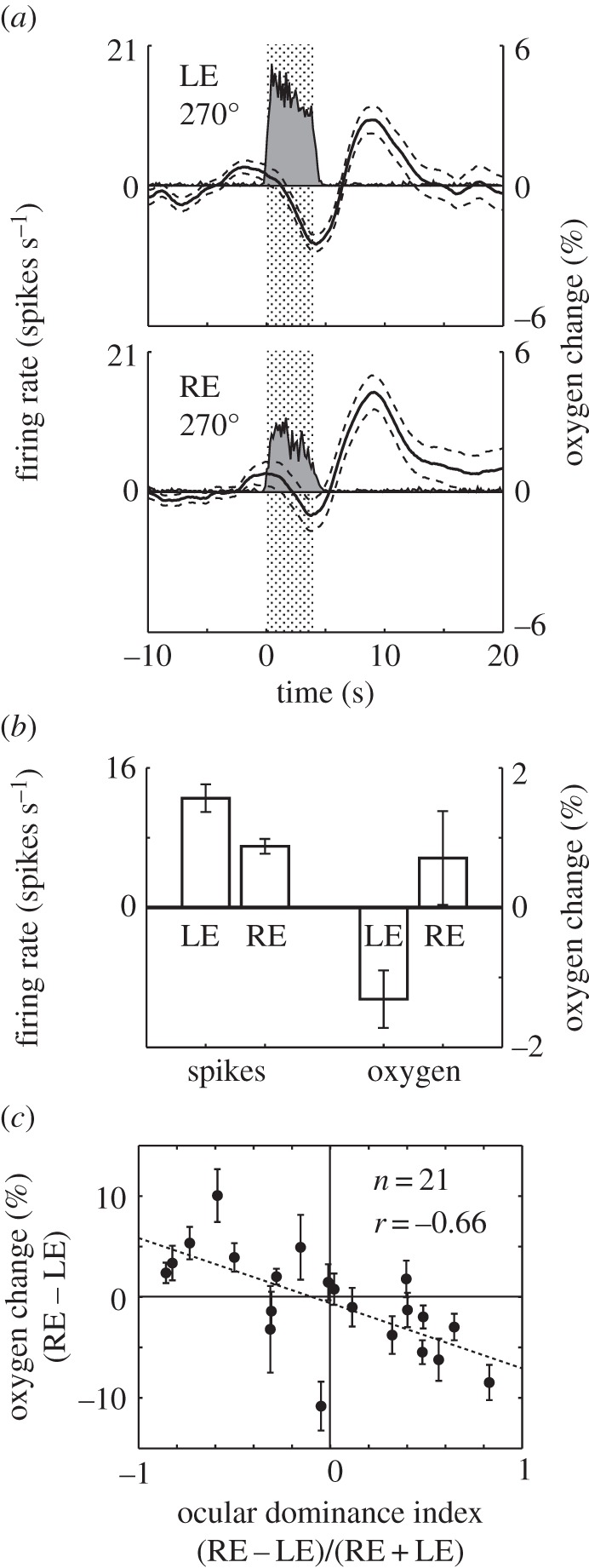
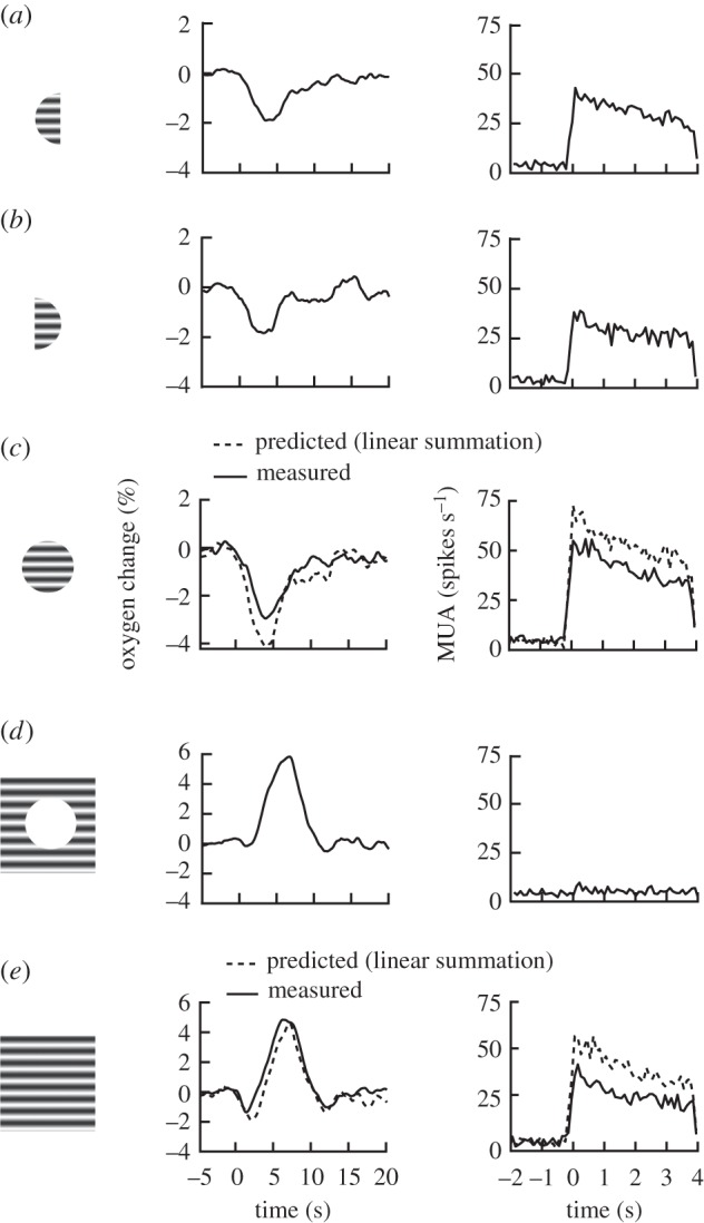
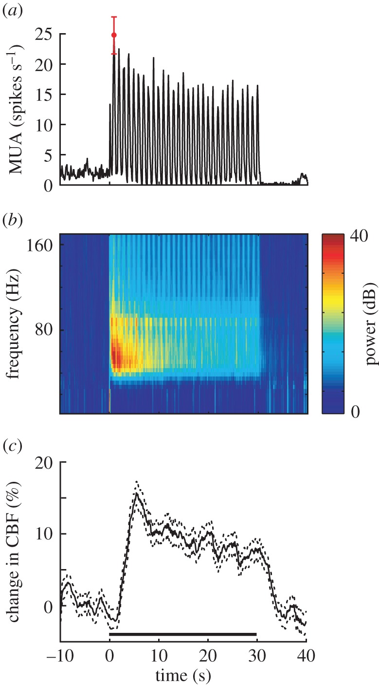
Studies are described which are intended to improve our understanding of the primary measurements made in non-invasive neural imaging. The blood oxygenation level-dependent signal used in functional magnetic resonance imaging (fMRI) reflects changes in deoxygenated haemoglobin. Tissue oxygen concentration, along with blood flow, changes during neural activation. Therefore, measurements of tissue oxygen together with the use of a neural sensor can provide direct estimates of neural-metabolic interactions. We have used this relationship in a series of studies in which a neural microelectrode is combined with an oxygen micro-sensor to make simultaneous co-localized measurements in the central visual pathway. Oxygen responses are typically biphasic with small initial dips followed by large secondary peaks during neural activation. By the use of established visual response characteristics, we have determined that the oxygen initial dip provides a better estimate of local neural function than the positive peak. This contrasts sharply with fMRI for which the initial dip is unreliable. To extend these studies, we have examined the relationship between the primary metabolic agents, glucose and lactate, and associated neural activity. For this work, we also use a Doppler technique to measure cerebral blood flow (CBF) together with neural activity. Results show consistent synchronously timed changes such that increases in neural activity are accompanied by decreases in glucose and simultaneous increases in lactate. Measurements of CBF show clear delays with respect to neural response. This is consistent with a slight delay in blood flow with respect to oxygen delivery during neural activation.This article is part of the themed issue 'Interpreting BOLD: a dialogue between cognitive and cellular neuroscience'.

Keywords: blood flow; glucose; lactate; neural activity; tissue oxygen; visual system.

Figure 1.

A dual neural–metabolic sensor. (a) A schematic configuration of the sensor. A neural microelectrode and an oxygen micro-sensor are enclosed in a double-barrel glass pipette. The tip of the neural electrode extends through the oxygen permeable membrane into tissue. The neural electrode and oxygen cathode are made of platinum. The oxygen anode is a silver–silver chloride reference electrode. (b) The sensor is displayed in brain tissue showing Golgi stained cells in the primate visual cortex. The spherical sensing field of the sensor is approximately 60 µm in diameter.

Figure 2.

Orientation selectivity of neural and tissue oxygen responses in visual cortex. (a) Neural and tissue oxygen responses to visual stimuli of different orientations for a representative recording site. Data are averaged responses across 72 trials. Oxygen responses are quantified as percentage change from baseline signals. Dashed lines represent ±1 s.e.m. (b) Orientation tuning curves of neural and tissue oxygen responses. The oxygen level is determined when oxygen and neural responses show maximum correlation (5.75 s after stimulus onset) for each orientation condition. Neural responses are quantified as the average spiking rates during the stimulus. Spontaneous activity is subtracted from neural responses for each orientation condition. Oxygen response is quantified as the percentage change from the baseline occurring 5.75 s after stimulus onset. Note that this time gives the best correlation between spike rate and tissue oxygenation for the group of data. Average spike and oxygen responses are fit to independent Gaussian functions. Error bars represent ±1 s.e.m. (c,d) Comparison of orientation selectivity between neural and oxygen responses for a group of recording sites (n = 16). Distributions of differences in preferred orientation (c) and tuning width (d) are shown between neural and oxygen responses. Downward arrows indicate mean values.

Figure 3.

Ocular dominance values of neural and oxygen responses. (a) Neural and oxygen responses for the same recording site as in figure 2 are shown for left eye ((a), top) and right eye ((a), bottom) stimulation. (b) Bar plots compare the average neural and oxygen responses (5.75 s after stimulus onset) between the two eyes. (c) The difference in oxygen change between the two eyes is plotted as a function of the ocular dominance index for a population of recording sites (n = 21). Each filled circle represents a recording site.

Figure 4.

Degree of temporal linearity of neurometabolic coupling in the LGN. (a,b) Neural and oxygen responses to visual stimuli of different durations (2 and 16 s) for a representative recording site. A small stimulus is centred over the receptive field (a), and a full-field stimulus with a blank mask covering the receptive field of the recording site (b). Dashed lines represent ±1 s.e.m. (c) Estimation of temporal linearity of tissue oxygen response. Predicted responses to long-duration stimuli are generated by replicating, shifting, and summing measured responses to short-duration stimuli. Blue and red lines indicate responses to small and large stimuli, respectively. Large stimulus contains mask over receptive field. Measured and predicted oxygen responses to 16 s stimuli based on 2 s stimuli are shown in solid and dashed lines, respectively.

Figure 5.

Degree of spatial linearity of neurometabolic coupling in the LGN. (a–c) Tissue oxygen and neural responses to visual stimuli of different spatial patterns within the receptive field for a recording site. A left semicircular stimulus (a), a right semicircular stimulus (b), and a full circular stimulus (c) are centred on the receptive field. Optimal receptive field size stimuli are used, and the sum of those in (a) and (b) is equal to that in (c). Oxygen and neural responses are shown in middle and right columns, respectively. (d) A full-field stimulus with a blank mask covering the receptive field is used to stimulate the surround. (e) A full-field stimulus. Summation of the stimuli in (c) and (d) matches the full-field stimulus (e). Data are averaged over 32 trials. Black and dashed curves in (c) and (e) represent measured and predicted composite oxygen and neural responses to the full circular receptive field stimulus (c) and the full-field stimulus (e), respectively.

Figure 6.

Binocular interaction profiles of neural and tissue oxygen responses for a representative recording site in striate cortex. (a–d) Averaged MUA (a), LFP (b), initial dip (c) and positive peak (d) of oxygen responses as a function of interocular spatial phase difference. Drifting sinusoidal gratings were presented to the two eyes to create interocular phase differences of: 0°, 60°, 120°, 180°, 240° and 300°. A monocular control stimulus to the dominant eye was included in the random sequence. Dashed lines in (a–d) represent responses to the monocular control stimulus. ‘0’ on the horizontal axes represents onset of the visual stimulus. Data are averaged across 48 trials. Mean LFP is averaged across a frequency range of 25–115 Hz. Error bars are ±1 s.e.m. (e–g) Normalized changes (C_n) for MUA, LFP and initial oxygen dip for recording sites with significant excitatory (facilitative) binocular interaction (n = 37). Each open circle represents a recording site. Comparisons of C_n between MUA and LFP (e), MUA and initial oxygen dip (f), and LFP and initial oxygen dip (g), respectively. (h) Average C_n for MUA, LFP and initial oxygen dip. Error bars represent ±1 s.e.m. (i–l) Normalized changes are given for MUA, LFP and initial oxygen dip for the condition of inhibitory (suppressive) binocular interaction (n = 29).

Figure 7.

Neural, glucose and lactate responses to visual stimuli. (a–c) Neural (spike discharge) (a), glucose (b) and lactate (c) responses to an optimal drifting sinusoidal grating at 10% contrast for a representative recording site. Data are averaged across 16 trials. The duration of visual stimuli is 30 s. The sampling rate for spiking activity is 25 kHz while that for glucose and lactate is 10 Hz. To compare temporal coupling between neural, glucose and lactate responses to visual stimulation, spiking activity is grouped at 10 Hz. The horizontal bar in (a) represents stimulus onset and duration. Error bars in (a–c) represent the maximum ±1  s.e.m. during visual stimulation. (d–f) Data in (a–c) are averaged across every five data points and re-plotted here. The temporal resolution is 2 Hz. (g) Contrast tuning functions for neural, glucose and lactate responses are given for the four contrast levels. A tight coupling is shown here between the three measurements. (h) Percentage changes of glucose and lactate signals are presented as a function of spiking rate. Absolute values are shown for changes in glucose responses (g,h). Dotted lines and error bars represent ±1  s.e.m.

Figure 8.

Simultaneous measurements of cerebral blood flow (CBF) and neural activity during presentation of optimal drifting sinusoidal grating. The stimulus size is 2°. The temporal and spatial frequencies are 1 Hz and 0.52 cycles per degree, respectively. (a,b) Neural responses exhibit a simple-cell pattern for MUA (a) and LFP (b), which show modulation in synchrony with the temporal frequency of visual stimulation. Error bar in (a) represents the maximum ±1  s.e.m. for MUA during visual stimulation. (c) CBF response to same visual stimulus. The CBF signal shows a sustained high-level change during visual stimulation. The sampling rate of the CBF signal is 10 Hz. The horizontal bar represents stimulus onset and duration (30 s). Dotted lines represent ±1  s.e.m.

References

1. Fox PT, Raichle ME. 1986. Focal physiological uncoupling of cerebral blood flow and oxidative metabolism during somatosensory stimulation in human subjects. Proc. Natl Acad. Sci. USA 83, 1140–1144. (10.1073/pnas.83.4.1140) - DOI - PMC - PubMed
1. Fox PT, Raichle ME, Mintun MA, Dence C. 1988. Nonoxidative glucose consumption during focal physiologic neural activity. Science 241, 462–464. (10.1126/science.3260686) - DOI - PubMed
1. Kim SG, Ogawa S. 2012. Biophysical and physiological origins of blood oxygenation level-dependent fMRI signals. J. Cereb. Blood Flow Metab. 32, 1188–1206. (10.1038/jcbfm.2012.23) - DOI - PMC - PubMed
1. Logothetis NK, Wandell BA. 2004. Interpreting the BOLD signal. Annu. Rev. Physiol. 66, 735–769. (10.1146/annurev.physiol.66.082602.092845) - DOI - PubMed
1. Davis TL, Kwong KK, Weisskoff RM, Rosen BR. 1998. Calibrated functional MRI: mapping the dynamics of oxidative metabolism. Proc. Natl Acad. Sci. USA 95, 1834–1839. (10.1073/pnas.95.4.1834) - DOI - PMC - PubMed
Publication types