A high-resolution time-depth view of dimethylsulphide cycling in the surface sea

Abstract

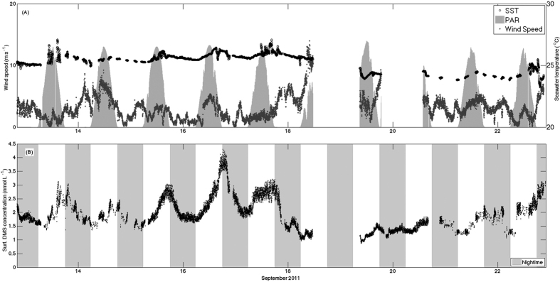
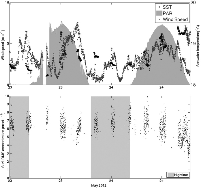
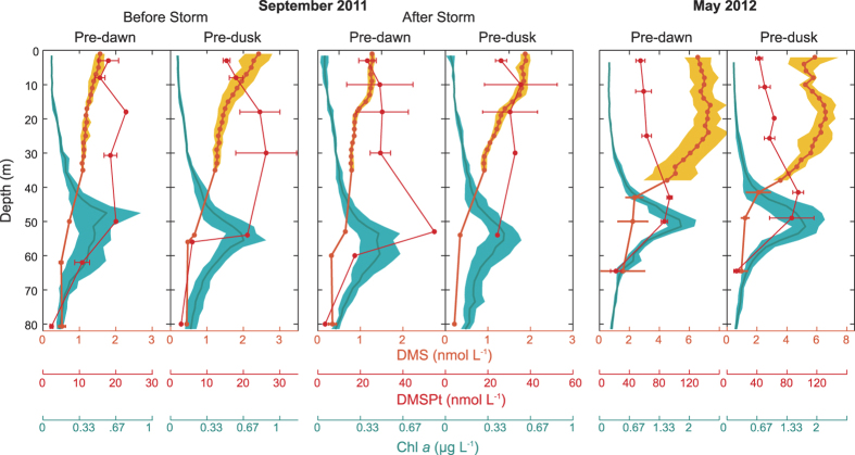
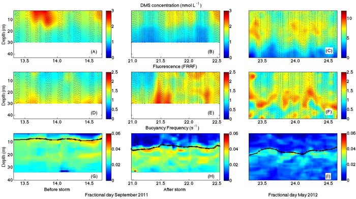
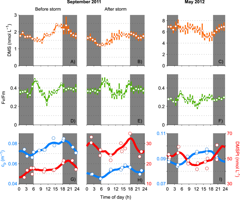
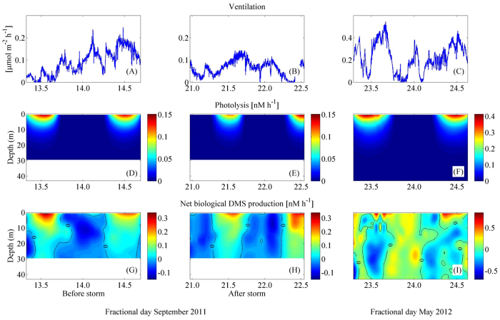
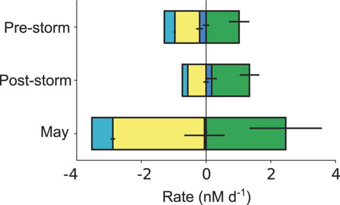
Emission of the trace gas dimethylsulphide (DMS) from the ocean influences the chemical and optical properties of the atmosphere, and the olfactory landscape for foraging marine birds, turtles and mammals. DMS concentration has been seen to vary across seasons and latitudes with plankton taxonomy and activity, and following the seascape of ocean's physics. However, whether and how does it vary at the time scales of meteorology and day-night cycles is largely unknown. Here we used high-resolution measurements over time and depth within coherent water patches in the open sea to show that DMS concentration responded rapidly but resiliently to mesoscale meteorological perturbation. Further, it varied over diel cycles in conjunction with rhythmic photobiological indicators in phytoplankton. Combining data and modelling, we show that sunlight switches and tunes the balance between net biological production and abiotic losses. This is an outstanding example of how biological diel rhythms affect biogeochemical processes.

Figure 1. Lagrangian series of DMS and physical forcing in the September 2011 cruise.

(A) Times series of wind speed (m s⁻¹ – dark grey); sea surface temperature (°C – black circles); and solar radiation in light grey (scaled; maximum irradiance of 1770 μmol photons m⁻² s⁻¹). (B) Time series of DMS surface concentrations (nmol L⁻¹). The shaded bars represent nighttime. The large data gaps on days 18–20 were due to a storm and instrumental problems.

Figure 2. As in Fig. 1 but for the May 2012 cruise.

Temperature and DMS data are not continuous because they were collected with the vertical profiler, which had to be stopped and drawn out of the water every time a CTD cast was taken.

Figure 3. Vertical patterns.

Averaged vertical profiles from the surface to below the deep chlorophyll maximum (DCM) for DMS (nmol L⁻¹), DMSP_t (nmol L⁻¹) and Chl-a (μg L⁻¹; fluorescence profiles calibrated with extracted chla measured in discrete bottles). DMS below 35 m and DMSP_t data are from discrete samples from CTD rosette. DMS above 35 m and chla profiles are 30 seconds means of measurements from the continuous vertical profiler, and standard deviations are indicated as shaded areas. Pre-dawn and pre-dusk profiles are shown for (A) 13–14 September before storm, (B) 21–22 September after storm, (C) May. The depth of the mixing layer is indicated in Fig. 4.

Figure 4. High-resolution time-depth distributions during the intensive Lagrangian studies.

The positions of the original data are shown as black dots in the foreground. Colors show data interpolation over 1 m and 1 min. (A–C) DMS concentrations (nmol L⁻¹), (D–F) chlorophyll a fluorescence from the FRRf, (G–I) buoyancy frequency (s⁻¹). Black lines on the buoyancy plots represent the mixing layer depth calculated from a 0.05 kg m⁻³ departure from the density at a reference depth of 2 m.

Figure 5. Characteristic diel cycles of DMS(P) and photobiological indicators in surface waters.

High-resolution DMS concentration (A–C) and photosystem II efficiency (Φ_PSII, D–F) binned to hourly frequency, plus total DMSP (DMSPt) concentration and beam attenuation due to particles (c_p) measured every four hours from CTD-Niskin bottle casts (panels G–I). The data represent upper mixed-layer averages from which the underlying two-day trend (if any) has been removed. Lines in G–I are spline fits smoothed with 4-h running means.

Figure 6. Computed rates for DMS cycling processes in the three intensive studies.

(Top) Ventilation rate (μmol m⁻² h⁻¹). (Middle) Photolysis rate (nmol L⁻¹ h⁻¹). (Bottom) Net biological production (nmol L⁻¹ h⁻¹).

Figure 7. Average mixed-layer budgets of DMS source (positive) and loss (negative) process rates and their associated uncertainties in the three intensive studies.

The 48-h averages are shown for ventilation (light blue), photolysis (yellow), vertical transport (dark blue) and net biological production (green). Numbers are given in Table S4.

References

1. Simó R. Production of atmospheric sulfur by oceanic plankton: biogeochemical, ecological and evolutionary links. Trends Ecol. Evol. 16, 287–294 (2001). - PubMed
1. Stefels J., Steinke M., Turner S. M., Malin G. & Belviso S. Environmental constraints on the production and removal of the climatically active gas dimethylsulphide (DMS) and implications for ecosystem modelling. Biogeochem. 83, 245–275 (2007).
1. Charlson R. J., Lovelock J. E., Andreae M. O. & Warren S. G. Oceanic phytoplankton, atmospheric sulphur, cloud albedo and climate. Nature 326, 655–661 (1987).
1. Andreae M. O. & Rosenfeld D. Aerosol–cloud–precipitation interactions. Part 1. The nature and sources of cloud-active aerosols. Earth-Science Rev. 89, 13–41 (2008).
1. Lovelock J. E., Maggs R. J. & Rasmussen R. A. Atmospheric dimethyl sulphide and the natural sulphur cycle. Nature 237, 452–453 (1972).
Publication types