The natural statistics of blur

Abstract

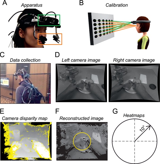
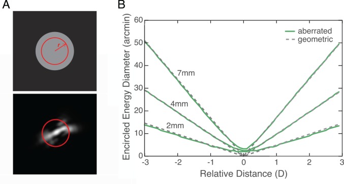
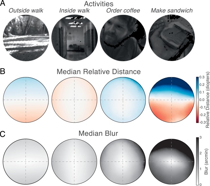
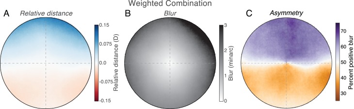
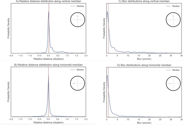
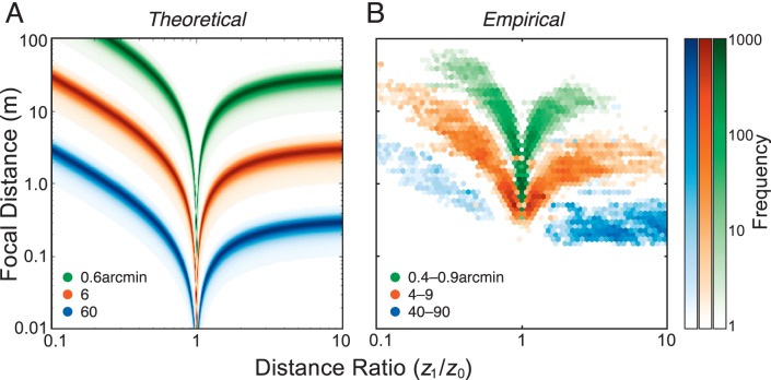
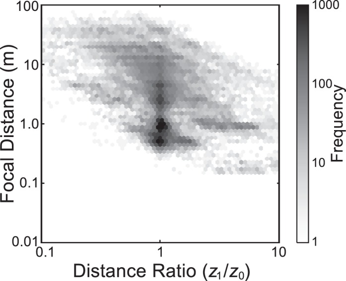
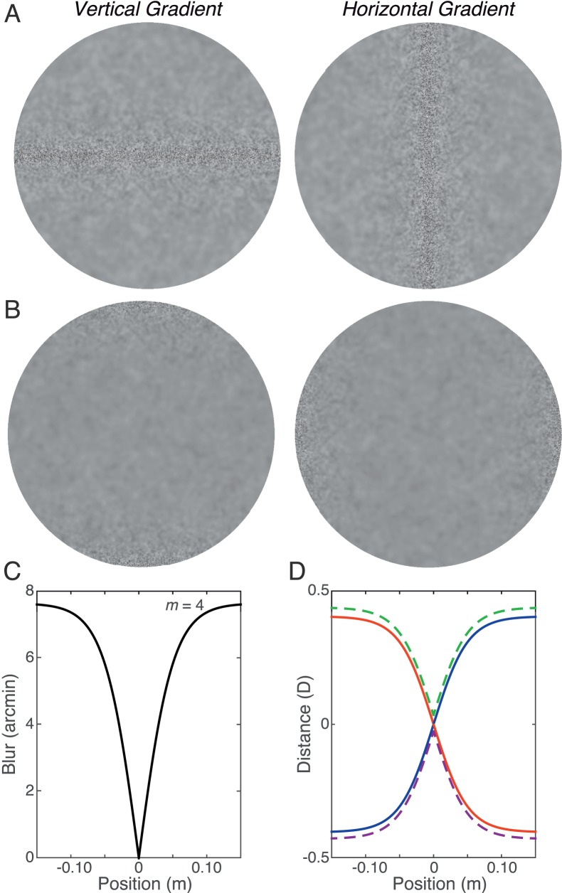
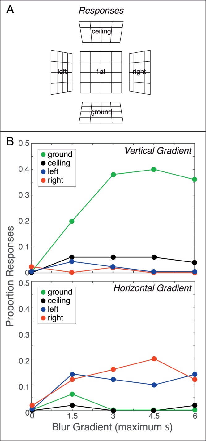
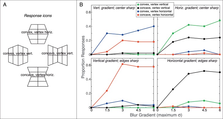
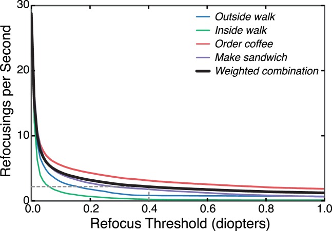
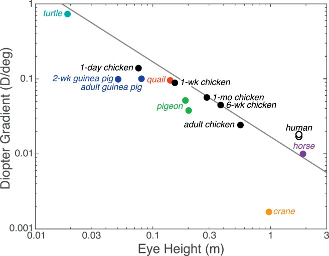
Blur from defocus can be both useful and detrimental for visual perception: It can be useful as a source of depth information and detrimental because it degrades image quality. We examined these aspects of blur by measuring the natural statistics of defocus blur across the visual field. Participants wore an eye-and-scene tracker that measured gaze direction, pupil diameter, and scene distances as they performed everyday tasks. We found that blur magnitude increases with increasing eccentricity. There is a vertical gradient in the distances that generate defocus blur: Blur below the fovea is generally due to scene points nearer than fixation; blur above the fovea is mostly due to points farther than fixation. There is no systematic horizontal gradient. Large blurs are generally caused by points farther rather than nearer than fixation. Consistent with the statistics, participants in a perceptual experiment perceived vertical blur gradients as slanted top-back whereas horizontal gradients were perceived equally as left-back and right-back. The tendency for people to see sharp as near and blurred as far is also consistent with the observed statistics. We calculated how many observations will be perceived as unsharp and found that perceptible blur is rare. Finally, we found that eye shape in ground-dwelling animals conforms to that required to put likely distances in best focus.

Figure 1

Defocus blur in a simple eye. z₀ is the focal distance of the eye given the focal length f and the distance from the lens to the image plane s₀. The relationship between these parameters is given by 1/s₀ + 1/z₀ = 1/f. Thus, f = s₀ when z₀ = infinity. An object at distance z₁ creates a blur circle of diameter b given the pupil diameter A.

Figure 2

Apparatus and method for determining defocus blur when participants are engaged in everyday tasks. (A) The apparatus. A head-mounted binocular eye tracker (orange box) was modified to include outward-facing stereo cameras (green box). Eye-tracking and stereo-camera data collection were synchronized, and disparity maps were computed offline from the stereo images. (B) Calibration. To determine the distances of scene points, we had to transform the image data in camera coordinates to eye-centered coordinates. The participant was positioned with a bite bar to place the eyes at known positions relative to a large display. A calibration pattern was then displayed for the cameras and used to determine the transformation between camera viewpoints and the eyes' known positions. (C) Apparatus and participant during data collection. Data from the tracker and cameras were stored on mobile computers in a backpack worn by the participant. (D, E) Two example images from the stereo cameras and a disparity map. Images were warped to remove lens distortion, resulting in bowed edges. The disparities between these two images were used to reconstruct the 3D geometry of the scene. Those disparities are shown as a grayscale image, with bright points representing near pixels and dark points representing far pixels. Yellow indicates regions in which disparity could not be computed due to occlusions and lack of texture. (F) The 3D points from the cameras were reprojected to the two eyes. The example is a reprojected image for the left eye. The yellow circle (20° diameter) indicates the area over which statistical analyses were performed. (G) Data are plotted in retinal coordinates with the fovea at the center. Upward in the visual field is upward and leftward is leftward. Azimuth and elevation are calculated in Helmholtz coordinates.

Figure 3

Encircled energy for aberrated eye and for cylinder approximation. (A) The point-spread function (PSF) for the cylinder function we used is shown in the upper panel. The PSF for an eye with typical aberrations is shown in the lower panel. Modeled pupil diameter was 3.5 mm, relative distance was −0.5D, and the light was equal-energy white. The red circles represent the circles used to calculate encircled energy. They have radii of r. (B) Diameters of circles that encircle 50% of the energy as a function of relative distance. A relative distance of 0 corresponds to perfect focus. The three sets of curves are for pupil diameters of 7, 4, and 2 mm. (Note that the PSF in the lower left panel is not for a condition on one of the green curves; instead, it lies between the 2- and 4-mm curves.) The solid green lines represent the encircled energy for the aberrated eye. The dashed gray lines represent them for the cylinder approximation.

Figure 4

Median relative distances and blur-circle diameters for each task. (A) Icons representing the four natural tasks. From left to right, they are outside walk, inside walk, order coffee, and make sandwich. (B) The medians of the relative-distance distributions (i.e., the difference between the distance to a scene point and the distance to the fixation point in diopters) are plotted for each point in the central 20° of the visual field. Upward in the panels is up in the visual field and leftward is left. Each panel shows the medians for the task above it combined across subjects. Blue represents positive relative distance (points farther than fixation), and red represents negative relative distance (nearer than fixation). The values at the top of the right panel are slightly clipped. (C) The medians of defocus blur for the four tasks. The median diameter of the blur circle is plotted for each point in the central visual field. Darker colors represent greater diameters. The values at the top of the right panel are slightly clipped.

Figure 5

Relative distance, blur, and asymmetry for the weighted combination of data across tasks. (A) The medians of the relative-distance distributions for the weighted combination of the data from the four tasks. Blue and red represent positive and negative relative distances, respectively. (B) Medians of blur for the weighted combination of data. Blur values are the diameters of the blur circle. Darker colors represent larger values. (C) Asymmetry. The percentages of blur observations that are associated with positive relative distance are plotted for each position in the visual field. Purple indicates values greater than 50% and orange values less than 50%.

Figure 6

Videos showing relative-distance and blur distributions near the vertical and horizontal meridians of the visual field. (A) Probability of different relative distances for a strip ±2° from the vertical meridian. The data are the weighted combination across tasks, averaged across subjects. The vertical dashed line indicates a value of 0. The vertical orange line represents the median relative distance for each elevation. The dot in the circular icon in the upper right indicates the position in the visual field for each distribution. (B) Probability of different relative distances for a strip ±2° from the horizontal meridian. The conventions are the same as in A. (C) Probability of different blur values along the vertical meridian. The data are the weighted combination across tasks and subjects. The vertical line represents the median. (D) Probability of different blur values along the horizontal meridian. The vertical line again represents the median.

Figure 7

The probability of different amounts of defocus blur given the distance to which the eye is focused (z₀) and the ratio of the object distance divided by the focal distance (z₁/z₀). (A) The theoretical probability distributions for different amounts of blur (green for 0.6 arcmin, orange for 6 arcmin, and blue for 60 arcmin). We assumed a Gaussian distribution of pupil diameters with a mean of 5.8 mm and standard deviation of 1.1 mm; these numbers are consistent with the diameters measured when our subjects were performing the natural tasks. Higher probabilities are indicated by darker colors. As the distance ratio approaches 1, the object moves closer to the focal distance. There is a singularity at a distance ratio of 1 because the object by definition is in focus at that distance. (B) The empirical distributions of focal distance and distance ratio given different amounts of blur. Different ranges of blur are represented by green (0.4–0.9 arcmin), orange (4–9 arcmin), and blue (40–90 arcmin). The number of observations for each combination of focal and relative distance is represented by the darkness of the color, as indicated by the color bars on the right. The data were binned with a range of ∼1/15 log unit in focal distance and ∼1/30 log unit in distance ratio.

Figure 8

The probability of different focal distances and distance ratios. The number of observations for each combination of focal distance and distance ratio is represented by the darkness of the color, as indicated by the color bar on the right. The data were binned with a range of ∼1/15 log unit in focal distance and ∼1/30 log unit in distance ratio.

Figure 9

Experimental stimuli and corresponding shapes. (A) White-noise textures with blur gradients. The one on the left has a vertical blur gradient and the one on the right a horizontal blur gradient. In both cases, the blur kernel was zero in the middle of the image and increased monotonically with eccentricity. (B) White-noise textures with blur gradients but with the blur kernel at zero at the edges of the stimuli. (C) Blur as a function of image position in the experimental stimuli with sharp centers. The value of m (Equation 3) is 4. We converted the Gaussian blur kernels with standard deviation σ into cylindrical blur kernels, so the ordinate is now the diameter of the corresponding cylinder. We made this conversion so that we could calculate the corresponding relative distances with Equation 2. (D) The 3D shapes that would create the blur distribution in panel C. Distance from fixation in diopters is plotted as a function of image position. There are four shapes that are consistent with the blur distribution: (1) a surface slanted top-back (blue), (2) a surface slanted top-forward (red), (3) a convex wedge (green dashed), and (4) a concave wedge (purple dashed). The dashed lines have been displaced slightly vertically to aid visibility.

Figure 10

Blur gradients and perception of planar 3D shape. (A) Response icons for five of the nine possible responses. These are the five planar responses. There were also four wedge responses (Figure 11A). (B) Experimental results with vertical and horizontal blur gradients; the upper panel is for vertical gradients and the lower for horizontal gradients. In both panels, the proportion of responses of a particular category (green for ground plane, black for ceiling plane, red for right-side forward, and blue for left-side forward) is plotted as a function of the magnitude of the blur gradient. The abscissa values are the maximum values of σ in Equation 6. The data have been averaged across the five observers. We calculated the departure of the data from equal distribution of responses among the geometrically plausible alternatives for each value of m. Specifically, we computed goodness-of-fit χ² for the observed responses relative to responses distributed equally among five alternatives. When the blur gradient was vertical, we considered observed responses relative to the alternatives of “flat,” “ground,” “ceiling,” “convex” (horizontal vertex), and “concave” (horizontal vertex). When the gradient was horizontal, we considered responses relative to “flat,” “left,” “right,” “convex” (vertical vertex), and “concave” (vertical vertex). All χ² values were statistically significant (p < 0.01), except for m = 1, horizontal gradient, sharp center. This means that responses were not randomly distributed among the planar alternatives.

Figure 11

Blur gradients and perception of wedge 3D shape. (A) Response icons for four wedge-like responses (four of nine possible responses). (B) Experimental results. The panels plot the proportion of responses of a particular category as a function of the magnitude of the blur gradient. The abscissa values are the maximum values of σ in Equation 3. The upper panels show the proportions of responses when the center of the stimulus was sharp and the edges blurred. The lower panels show the response proportions when the edges were sharp and the center blurred. The left panels show the responses when the blur gradient was vertical. The right panels show them when the gradient was horizontal. The data have been averaged across the five observers. We calculated the departure of the data from equal distribution of responses among the geometrically plausible alternatives for each value of m. Specifically, we computed χ² for the observed responses relative to responses distributed equally among three alternatives. When the blur gradient was vertical, we considered observed responses relative to the alternatives of “flat,” “convex” (horizontal vertex), and “concave” (horizontal vertex). When the gradient was horizontal, we considered responses relative to “flat,” “convex” (vertical vertex), and “concave” (vertical vertex). All χ² values were statistically significant (p < 0.01), which means that responses were not randomly distributed among the alternatives.

Figure 12

Blur and the interpretation of 3D shape. The panels are photographs of a Necker cube with a pencil running through it. The camera was focused on the nearest vertex of the cube in the upper panel and on the farthest vertex in the lower panel. Photograph provided by Jan Souman.

Figure 13

Blur-detection threshold as a function of retinal eccentricity. Detectable changes in defocus are plotted as a function of retinal eccentricity. The left ordinate shows the changes in diopters and the right ordinate the changes in minutes of arc using a 5-mm pupil. The blue points are from Wang and Ciuffreda (2004); they reported the full depth of field, so we divided their thresholds by two. The red points are from Wang and Ciuffreda (2005) and the green points from Wang et al. (2006). The dashed line is the best linear fit to the data.

Figure 14

The percentage of detectable blurs across the visual field. (A) Percentage of detectable blur magnitudes in the central visual field for the four tasks. The diameter of the circles is 20° and the fovea is in the center. Darker colors represent higher percentages (see color bar on far right). (B) Percentage of detectable blur magnitudes in the central visual field for the weighted combination across tasks.

Figure 15

Percentage of detectable blurs with random fixations. Percentage of detectable blur magnitudes for the weighted combination of the four tasks combined across subjects when gaze directions are random. Darker colors represent higher percentages. The data at the bottom of the panel are slightly clipped.

Figure 16

Medians and standard deviations of relative distance with real and random fixations. (A) Median relative distances in the upper and lower fields plotted as a function of radial distance from the fovea. The medians were computed from all relative distances within the semicircular sampling window. The red and blue curves represent the data from the upper and lower fields, respectively. Solid and dashed curves represent the data from real and random fixations, respectively. (B) Standard deviations of relative distances in the upper and lower fields as a function of distance from fovea. The red and blue curves represent data from the upper and lower fields, respectively. Solid and dashed curves represent data from real and random fixations, respectively.

Figure 17

Refocusings required for different thresholds. The estimated number of refocusings per second is plotted as a function of the change in diopters that require a refocus response. The thin colored curves represent those values for each of the individual tasks averaged across subjects. The thick black curve represents those values for the weighted combination of data across the tasks, again averaged across subjects. The dashed lines indicate the number of refocusings needed if the refocus threshold is 0.4 diopters.

Figure 18

Image formation when the object is a slanted plane. z₀ is the focal distance of the eye measured along the optical axis. f is the focal length and s₀ is the distance from the lens to the plane of best focus along the optical axis. The object plane is slanted by θ relative to frontoparallel. A point on the object plane at distance z forms an image at distance s from the lens. The image is formed in a plane slanted by ϕ relative to frontoparallel.

Figure 19

Geometry of object and ground planes for an upright viewer. An eye at height h from the ground views a point on the ground at distance d. The line of sight is at angle θ relative to earth vertical. The ground plane is rotated by θ relative to a frontoparallel plane. The distance of the fixated point along the line of sight is z₀. For a point slightly lower in the visual field, but also on the ground, the distance is z₁. The angular difference between the vectors z₀ and z₁ is ε.

Figure 20

Relationship between eye height and lower-field myopia in ground-dwelling animals. The change in best focus as a function of elevation is plotted as a function of the typical height of the eye above the ground. The change in best focus is diopters per degree of elevation. To compute these values, we found the best-fitting line to data on refraction as a function of elevation. Turtle: figure 3 in Henze et al. (2004); spherical equivalent measured in three animals at 19 eccentricities across 55° of elevation. One-week and 1-month chicken: figure 6 in Schaeffel et al. (1994); refractive state in three 1-week and six 1-month chickens; measured at two eccentricities across 80° of elevation. One-day, 6-week, and adult chicken: table 2 in Hodos and Erichsen (1990); refractive state in three 1-day, three 6-week, and three adult chickens; two eccentricities across 60°. Two-week and adult guinea pig: table 2 in Zeng et al. (2013); spherical equivalent measured in 18 eyes of 2-week-olds and 31 eyes of adults; two eccentricities across 60°. Quail: table 2 in Hodos and Erichsen (1990); refractive state in five adult quails; two eccentricities across 60°. Pigeon: figure 4 in Fitzke et al. (1985); refractive state measured in 72 eyes; numerous eccentricities across 130°. Figure 5.16 in García-Sánchez (2012); spherical equivalent measured in eight eyes at 13 eccentricities across 60° (averaged across three azimuths). Crane: table 2 in Hodos and Erichsen (1990); refractive state in four adult cranes; measured at two eccentricities across 60° of elevation. Horse: table 2 in Sivak and Allen (1975); refractive state measured in four eyes at three eccentricities across 60°. Human: figure 3 from Seidemann et al. (2002); spherical equivalent measured in 62 eyes at nine eccentricities across 55°. Table 2B in Ehsaei et al. (2011); refractive state in 36 emmetropic eyes; measured at seven eccentricities across 60°. Eye height was either provided in the reference on refraction or was estimated from sources on the Internet. The line represents the prediction of the image plane of best focus if it were conjugate with the ground (Equation 16).

References

1. Banks M. S,, Sprague W.W,, Schmoll J,, Parnell J.A,, Love G.D. (2015). Why do animal eyes have pupils of different shapes? Science Advances, 1 (7), e1500391. - PMC - PubMed
1. Brisson J,, Mainville M,, Mailloux D,, Beaulieu C,, Serres J,, Sirois S. (2013). Pupil diameter measurement errors as a function of gaze direction in corneal reflection eyetrackers. Behavior Research Methods, 45, 1322–1331. - PubMed
1. Burge J,, Geisler W.S. (2011). Optimal defocus estimation in individual natural images. Proceedings of the National Academy of Sciences, USA, 108, 16849–16854. - PMC - PubMed
1. Campbell F. W. (1957). The depth of field of the human eye. Optica Acta, 4, 157–164.
1. Campbell F. W,, Westheimer G. (1958). Sensitivity of the eye to differences in focus. Journal of Physiology, 143, 18P.