. 2016 Sep 1:7:12682.
doi: 10.1038/ncomms12682.

Temporal asymmetries in auditory coding and perception reflect multi-layered nonlinearities

Affiliations

Temporal asymmetries in auditory coding and perception reflect multi-layered nonlinearities

Thomas Deneux et al. Nat Commun. .

Abstract

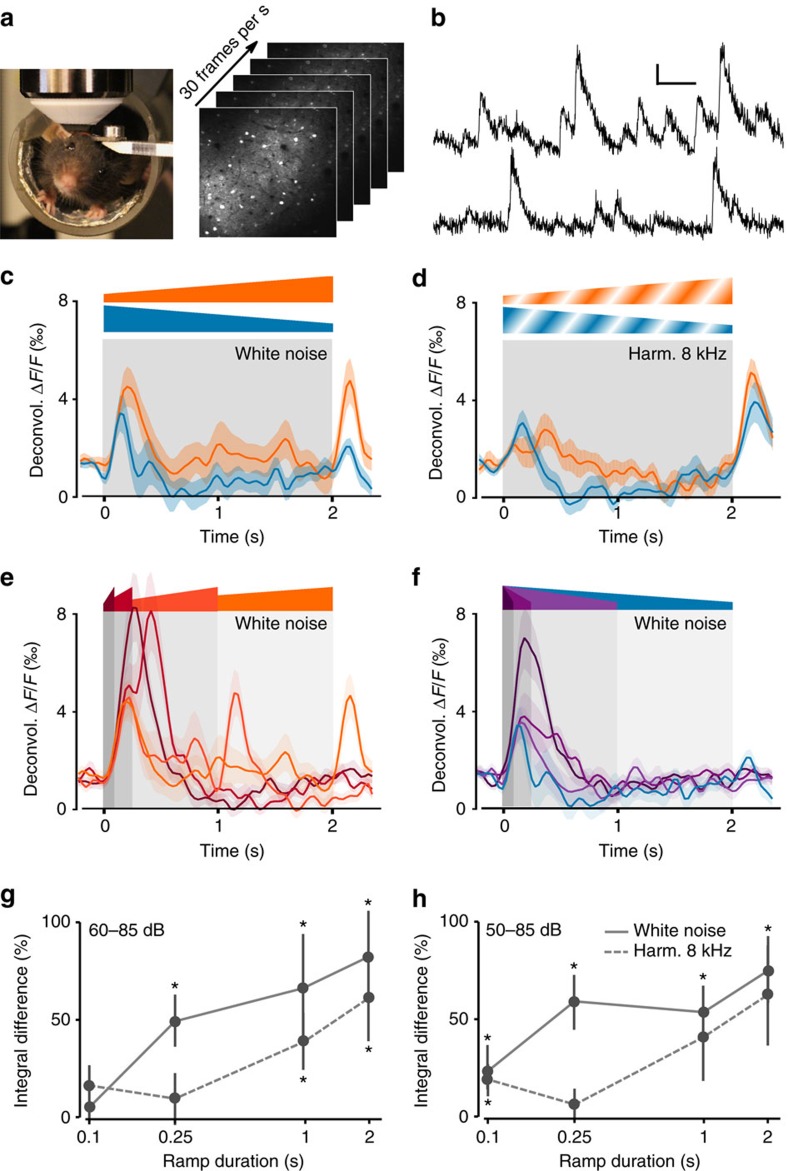
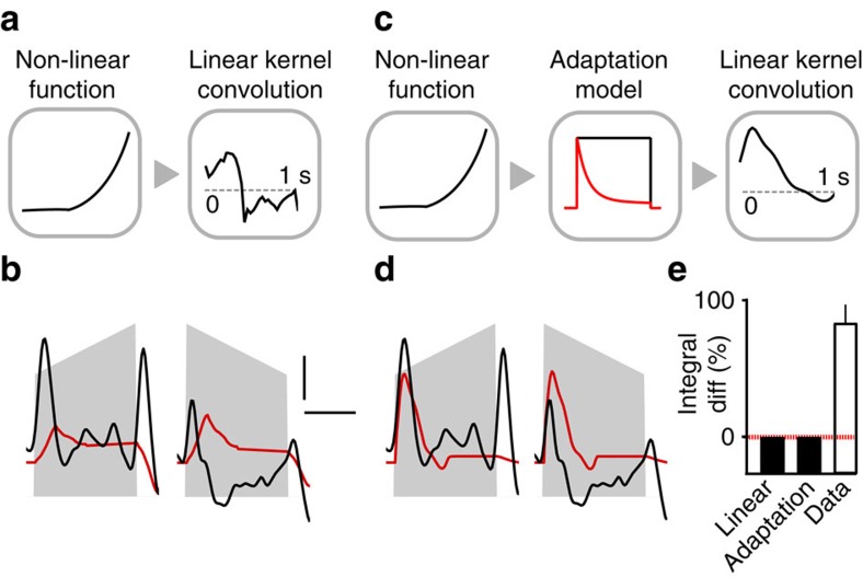
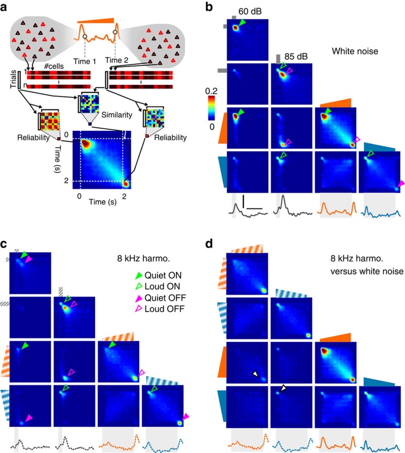
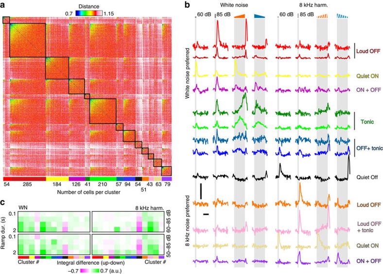
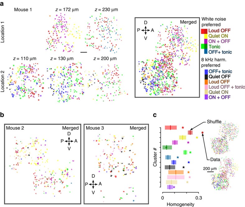
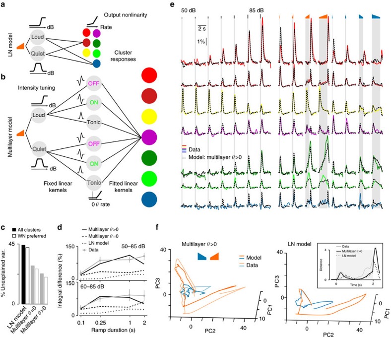
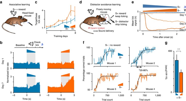
Sound recognition relies not only on spectral cues, but also on temporal cues, as demonstrated by the profound impact of time reversals on perception of common sounds. To address the coding principles underlying such auditory asymmetries, we recorded a large sample of auditory cortex neurons using two-photon calcium imaging in awake mice, while playing sounds ramping up or down in intensity. We observed clear asymmetries in cortical population responses, including stronger cortical activity for up-ramping sounds, which matches perceptual saliency assessments in mice and previous measures in humans. Analysis of cortical activity patterns revealed that auditory cortex implements a map of spatially clustered neuronal ensembles, detecting specific combinations of spectral and intensity modulation features. Comparing different models, we show that cortical responses result from multi-layered nonlinearities, which, contrary to standard receptive field models of auditory cortex function, build divergent representations of sounds with similar spectral content, but different temporal structure.


Figures

Figure 1
Figure 1. Asymmetry of responses to intensity ramps in mouse auditory cortex.
(a) Awake head-fixed mouse under the two-photon microscope and an example of a recorded image time series of GCAMP6s labelled neurons in cortical layer 2/3 of the mouse auditory cortex. (b) Examples of raw GCAMP6s signals for one neuron (sampling rate: 31.5 Hz). Scale bars, vertical 20% ΔF/F, horizontal 5 s. (c) Mean deconvolved calcium signals (that is, estimated firing rate) for 2 s white noise up- and down-ramps (range 60–85 dB SPL, shading indicates s.e.m. across n=15 imaging sessions). (d) Same as c for 2 s 8 kHz harmonic sound ramps (n=13 imaging sessions). (e) Responses to white noise up-ramps of 100 ms, 250 ms, 1 and 2 s. (f) Same as e for down-ramps. (g,h) Differences of the integrals of response signals between up and down-ramps (for example, integral of the difference of the two mean signals shown in c). The differences are normalized by the down-ramp integral. Error bars, s.e.m. When assessed globally (pooling durations together), the integral differences for each intensity range and spectral content was very significantly positive (Wilcoxon signed-rank test, white noise 60–85 dB: P=2 × 10⁻⁵, 50–85 dB: P=7 × 10⁻⁹ n=60 measurements; 8 kHz 60–85 dB: P=1 × 10⁻³, 50–85 dB: P=2 × 10⁻³, n=52 measurements). Statistical significance for individual stimuli is assessed across imaging sessions (white noise: n=15, 8 kHz: n=13) using the single-sided Wilcoxon rank-sum test and a Benjamini–Hochberg correction for multiple testing applied to the 16 tests (*P<0.05).
Figure 2
Figure 2. Cortical response asymmetry is a nonlinear effect.
(a) Sketch of the linear filter model. The input signal is scaled by a nonlinear function (left) and then goes through a linear kernel (right) to obtain the neuronal response. (b) Best fit by the linear model of the population responses to the 2 s white noise up- and down-ramps. Scale bars, vertical 0.1% ΔF/F, horizontal 1 s. (c) Sketch of the adaption model. The input signal is scaled by a nonlinear function (left), then undergoes adaptation (middle) and finally passes through a linear kernel (right). (d) Best fit by the adaptation model of the population responses to the 2 s white noise up- and down-ramps. (e) Integral differences between up- and down-ramps for the linear and adaptation models for any choice of parameters and any ramp waveform (analytical result) versus experimental integral differences for the 2 s white noise ramps.
Figure 3
Figure 3. Cortical population dynamics during up- and down-ramps.
(a) Schematic of the population vector similarity measure (Methods). For this analysis, we pooled all recorded neurons in a pseudo-population. The similarity between two population activity patterns (for example, patterns at time 1 and 2 post stimulus) corresponds to the average of all pair-wise correlations computed across single-trial population vectors. The reliability of a pattern is computed identically based on correlations computed across all single-trial occurrences of this pattern. (b) Population similarity matrix across time bins and stimuli for four white noise sounds (60 and 85 dB 0.25 s duration and 60–85 dB 2 s duration up- and don-ramps). Underneath the population firing rate waveforms are shown. The arrowheads on the diagonal indicate distinct activity patterns identified as ‘Quiet ON' (filled green), ‘Loud ON' (empty green), ‘Quiet OFF' (filled magenta) and ‘Loud OFF' (empty magenta). Arrowheads off the diagonal indicate strong similarities between different responses (for example, empty magenta arrowhead indicates similarity between ‘Loud OFF' activity patterns observed after the 85 dB 250 ms sound and after the 60–85 dB up-ramp). Scale bars, vertical 0.4% ΔF/F, horizontal 1 s. (c) Same as b for the harmonic 8 kHz tone. (d) Same as b and c, but the response to the white noise and 8 kHz ramps are compared.
Figure 4
Figure 4. Clustering of single neuron population responses.
(a) Distance matrix for the 1,341 clustered neurons. The metric used is d=1−cc, where cc stands for the Pearson correlation coefficient between response traces. The identified clusters are delineated by a black square and labelled at the bottom of the matrix by a coloured bar under which the number of cells in the cluster is indicated. Within each cluster the cells are sorted according to their mean distance with all other cells of the matrix. The gradient of distances within each cluster reflects the heterogeneity of the signal-to-noise ratio across cells. More reliable cells are on the left, less reliable cells on the right. (b) Mean response profiles of the 12 identified clusters to four white noise and 8 kHz harmonic sounds (60 and 85 dB 0.25 s duration and 60–85 dB 2 s duration up- and down-ramps). Scale bars, vertical 4% ΔF/F, horizontal 1 s. (c) Average absolute integral differences between up- and down-ramps for each cluster, ramp intensity ranges and durations.
Figure 5
Figure 5. Functional cell types correspond to cell assemblies clustered in space.
(a) Localizations of the cells belonging to the different identified clusters, colour-coded as in Fig. 4 (see colour bar on the right), in five imaging sessions performed at two different horizontal localizations and different depths (z) across several days in mouse 1. On the right, the relative localization of all cells is shown in a horizontally mapped z projection. Scale bar, 100 μm. (b) Horizontally mapped z projection for mouse 2 and mouse 3 (four imaging sessions each, Supplementary Fig. 4). (c) Each star represents the value of a homogeneity index calculated across three mice for each of the 13 clusters (same colour code as in a). The vertical lines represent the value expected if each cluster was homogenously spread in space obtained by shuffling and the shaded area is the 95% confidence interval. Maps obtained before and after shuffling are shown for one example mouse: note that cell shufflings are operated within individual mice, but homogeneity indexes averaged over neurons across all mice.
Figure 6
Figure 6. Phenomenological model of intensity modulation coding.
(a) Linear–nonlinear (LN) model (linear filters+output nonlinearity) applied to two different ‘intensity channels' obtained by nonlinear scaling of the input for intensity tuning. (b) The multilayer model with: (1) intensity channel as in a, (2) six fixed linear filters with a rectifying nonlinearity (threshold=θ) and (3) linear sum of the feature detector outputs filtered by fitted kernels. (c) Fraction of unexplained variance for all clusters (filled bars) or for the seven clusters preferring white noise (empty bars) after fitting the LN model, and the full multilayer model with a fixed (multilayer θ=0) or a fitted (multilayer θ>0) rectifying threshold. (d) Normalized difference of the up- and down ramp responses for the clustered data (1,341 neurons, n=13 imaging session) and the different fitted models as in b. (e) Fit of the multilayer model (θ>0) to the responses of the six identified clusters that show preferred response to white noise (note that all 12 clusters where fitted by the model). Sounds are white noise: 250 ms constant (seven intensities) and 60–85 dB up- and down-ramps. Scale bars, vertical 1% ΔF/F, horizontal 2 s. (f) Trajectories of the population responses to the 2 s white noise up- (orange) and down-ramps (blue) obtained for the fitted LN (right), the multilayer model and the data (left). The 13-dimensional data and model outputs are plotted in the space of the three first-principle components of the data. The trajectories are more divergent for the multilayer model than for the LN model, as corroborated by distance between the two trajectories at every time point (inset).
Figure 7
Figure 7. Up-ramps are behaviourally more salient than down-ramps.
(a) Sketch of the head-fixed sound-reward association task. (b) Histograms of lick rates normalized to the baseline rate during the first and seventh days of training to the up- (right) and down-ramps (left). Average across all mice (n=6 per group). (c) Ratio of the post- and pre-stimulus lick rates over training days for the up- (blue) and down-ramps (orange) (mean±s.e.m.), showing increased sound-locked licking for up-ramps, Friedman test, P=3.7 × 10⁻¹⁰, n=6 per group). (d) Schematic of the distractor avoidance learning task. Freely moving mice first learn to lick at a spout after an S+ sound to get a reward, then an S− sound is added and mice learn to stop licking after this sound. (e) Typical average infrared beam break signal (5 V=beam broken, 0 V=beam intact) with respect to S+ and S− sound onsets for a mouse on the first, second and fifth training days. (f) Examples of global performance learning curves (mean of S+ and S− performance) for the Go/NoGo distractor avoidance task. (g) Learning phase duration when either the down- (left) or the up-ramp (right) is the S− stimulus (mean±s.e.m., n=12 per group, P=0.0046, Kolmogorov–Smirnov test). The learning phase duration if defined as the time necessary to go from 20 to 80% of maximum performance above chance level (that is, >50% correct) and is measured on the sigmoid fitted to the learning curve.

Similar articles

Cited by

References

    1. Helmholtz H. v. & Ellis A. J. On the Sensations of Tone as a Physiological Basis for the Theory of Music 2nd edn Longmans, Green (1885).
    1. Lewis J. W. et al.. Human brain regions involved in recognizing environmental sounds. Cereb. Cortex. 14, 1008–1021 (2004). - PubMed
    1. McBeath M. K. & Neuhoff J. G. The Doppler effect is not what you think it is: dramatic pitch change due to dynamic intensity change. Psychon. Bull. Rev. 9, 306–313 (2002). - PubMed
    1. Nelken I., Rotman Y. & Bar Yosef O. Responses of auditory-cortex neurons to structural features of natural sounds. Nature 397, 154–157 (1999). - PubMed
    1. Theunissen F. E. & Elie J. E. Neural processing of natural sounds. Nat. Rev. Neurosci. 15, 355–366 (2014). - PubMed

Publication types

LinkOut - more resources