The Second Spiking Threshold: Dynamics of Laminar Network Spiking in the Visual Cortex

Abstract

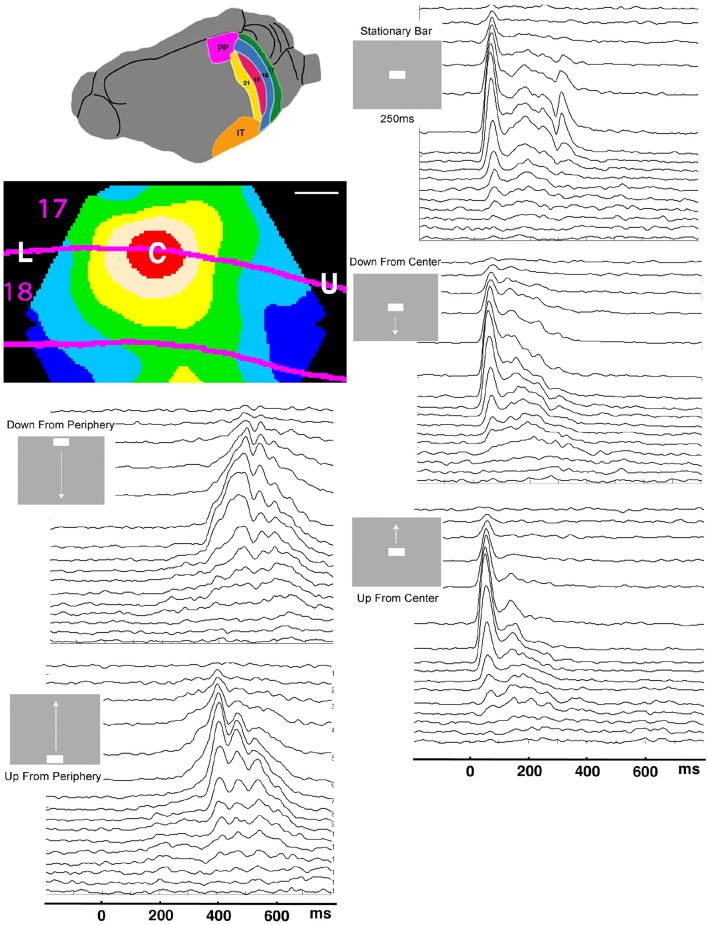
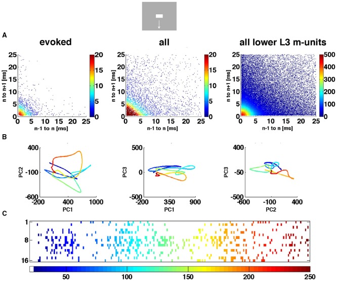
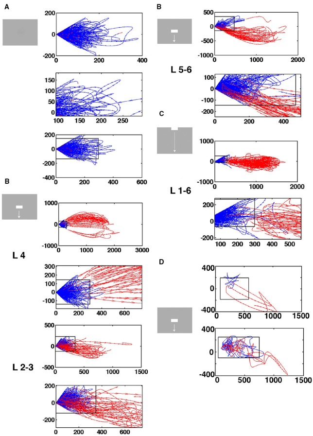
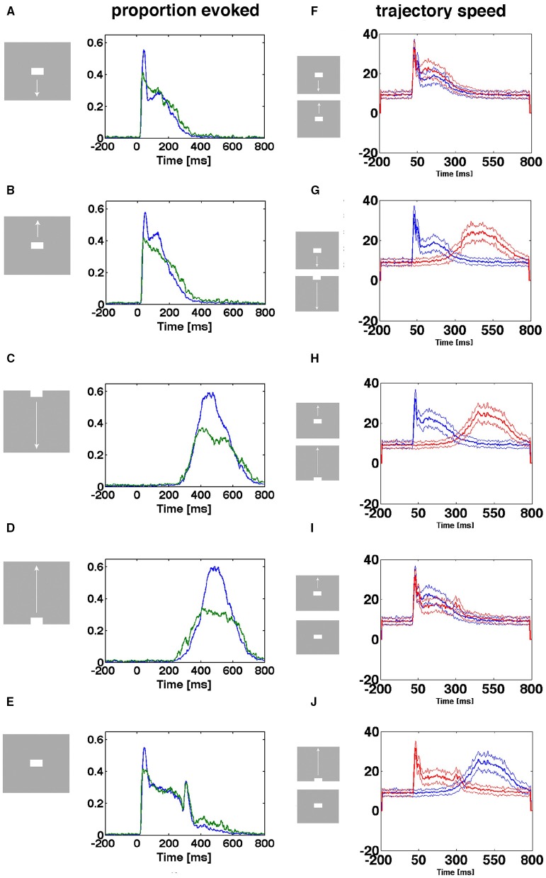
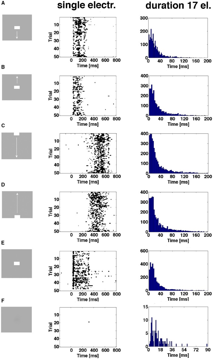
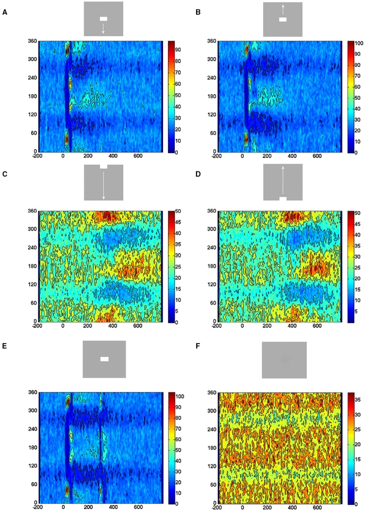
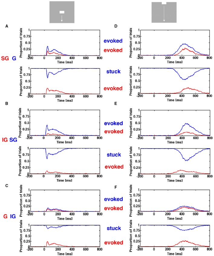
Most neurons have a threshold separating the silent non-spiking state and the state of producing temporal sequences of spikes. But neurons in vivo also have a second threshold, found recently in granular layer neurons of the primary visual cortex, separating spontaneous ongoing spiking from visually evoked spiking driven by sharp transients. Here we examine whether this second threshold exists outside the granular layer and examine details of transitions between spiking states in ferrets exposed to moving objects. We found the second threshold, separating spiking states evoked by stationary and moving visual stimuli from the spontaneous ongoing spiking state, in all layers and zones of areas 17 and 18 indicating that the second threshold is a property of the network. Spontaneous and evoked spiking, thus can easily be distinguished. In addition, the trajectories of spontaneous ongoing states were slow, frequently changing direction. In single trials, sharp as well as smooth and slow transients transform the trajectories to be outward directed, fast and crossing the threshold to become evoked. Although the speeds of the evolution of the evoked states differ, the same domain of the state space is explored indicating uniformity of the evoked states. All evoked states return to the spontaneous evoked spiking state as in a typical mono-stable dynamical system. In single trials, neither the original spiking rates, nor the temporal evolution in state space could distinguish simple visual scenes.

Keywords: dynamical systems; evoked activity; object vision; spontaneous activity; visual motion.

Figure 1

Laminar post-stimulus-histograms of the multiunit spiking to a single moving bar. Top left: posterior visual areas of the ferret. PP, posterior parietal; IT, inferior temporal. Below: Mean voltage sensitive dye signal of 7 animals 100 ms after appearance of a stationary bar at the CFOV. Red: C, zone mapping bar at CFOV; beige: edge zone; The lower part of the visual field is mapped between L and C, the upper visual field between C and U. Scale bar: 500 μm. Time scale 0 = start of stimulus. The smoothed (σ = 10 ms) spike rates from all 16 leads in all 5 stimulus conditions have identical time scales. The layer 1 lead recordings are in the top of the panels.

Figure 2

Nissl stained section of the posterior part of the brain of animal 4. The two yellow circles and the red circle show the cannula made holes used for the alignment of the slices. The red, yellow, and green cross, mark the borders between areas 17/18, 18/19, and 19/21. The detailed cytoarchitecture should be seen in higher resolution. The slices were reconstructed to a volume with the areal borders on the surface.

Figure 3

Temporal spiking dynamics. The color coded trajectories in 3-dimensional state space made by the axes of the first 3 principal components show the spiking dynamics of each condition (Materials and Methods) for the 4 electrode penetrations shown, one from each of the 4 cortical zones shown in the insert. (A) Maps the bar moving down from the peripheral FOV (early) and the bar moving up from the peripheral FOV (late), plus the bar moving up from the CFOV. (B) Maps the bar moving up from the peripheral FOV (early) and the bar moving down from the peripheral FOV (late), plus the bar moving down from the CFOV. (C) Maps all bars in or passing through the CFOV. (D) Maps all moving bars (The stationary bar, flashed in the CFOV produce a minor initial spiking here). The trajectories are composed of points, one for each ms, from which the speed by which the dynamics evolves can be appreciated. Note the chaotic-like evolution of the trajectories of all conditions in the pre-stimulus period and how the speed increases when the stimulus transients influence dynamics. The first 3 PCAs accounted for 64–83% of the variance. The values on the axes are in units of the principal components. The fixed point is located at (0,0,0).

Figure 4

The spiking dynamics reflect the collective spiking in all cortical layers. (A) Plot of inter-spike intervals of lower layer 3 multi-units located in the CFOV mapping zone. Left: inter-spike intervals (n = 1263), from evoked trials only, in ms from a single electrode penetration in response to a bar moving down from the CFOV. Middle: same electrode penetration inter-trial intervals (n = 5207) for all trials for the bar moving down from the CFOV. Right: inter-spike intervals (n = 30.774) for all lower layer 3 leads in the cortex mapping the CFOV. Note the absence of any periodicity. The color scales show the number of observations within 0.5 × 0.5 ms space. (B) Trajectory of a single trial (trial 30), from 0 to 250 ms in 3 different projections of state space generated by PCA color coded in time after stimulus to compare with (C). First 3 components accounted for 77% of total variance. (C) Same trial as (B), all spikes from all leads. All figures, except (B) left from animal 6, electrode penetration 2.

Figure 5

Separatrices in all cortical layers. Velocity vectors per ms in state space made by the first 2 principal components of the spiking from single electrode penetrations. (A) Spontaneous ongoing spiking. Note that all vectors at a certain distance bend from pointing outwards from the fixed point to point back to the fixed point from another angle. (B) Separatrices for bar moving down from CFOV. The separatrix also separates pre-stimulus velocity vectors pointing toward the fixed point from vectors showing flow in the opposite direction in evoked trials in the granular layer 30–50 ms after stimulus start (zoomed part of state space). Similar separatrices in layers 2–3 and 5–6 (B repeated). (C) Separatrices for bar moving down from peripheral FOV. Separatrix determined from collective spiking in all layers by diverging vector flows in pre-stimulus time and when trials became evoked 350–450 ms. (D) Top: Vector flow from 1 trial where the trajectory returns quickly toward the fixed point-for thereafter to be evoked again. Below: One evoked trial and two stuck stimulus trials. The values on the axes are those from the first (x-axis) and second (y-axis) principal components.

Figure 6

Two ways of entering the evoked state. Proportion evoked trials and trajectory speeds as functions of time from 17 electrode penetrations in the cortex mapping the CFOV. Stimulus start 0 ms. (A,B,E) Stimuli appearing in CFOV elicit sharp transients that swiftly brings the spiking into the evoked states. (C,D) For stimuli appearing outside the CFOV, the dynamics of the cortex initiate smoothly raising spiking dynamics gradually increasing trajectory speed and proportion evoked. Blue curves: mean proportion of trials evoked, green curves: square-root of variance. (F) Up and down moving bars appearing in CFOV give sharply increasing trajectory speeds. (G,H,J) Bars appearing first in peripheral field of view are mapped later with smoothly increasing trajectory speeds. (I) Stationary and moving bar appearing in CFOV have similar trajectory speeds. (J) A stationary bar and a bar passing the CFOV have different trajectory speeds. Note the correspondence between speeds and proportion-evoked trials. Mean thick curve, square root of variance thin curves.

Figure 7

Transitions from spontaneous spiking to evoked spiking: vector flow. (A) Transition from chaotic-like vector flow to evoked vector flow at the blue-red transition (animal 2). (B) Two trial transitions at 25 ms and one re-entry. Note also the transition of one of the trials in the pre-stimulus period (blue vectors) bending off at the separatrix. (C) Acceleration of trajectory speeds prior to the first entry into the evoked state after 20 ms post stimulus. All evoked trials from the 17 electrode penetrations mapping the CFOV. Yellow: mean speed; dark-blue stippled lines: 10%-ile and 90%-ile. A few trials were evoked prior to the sharp transient. X-axis: time prior to the crossing of the separatrix. Y-axis speed in state space. (D) Smooth transient driven acceleration of trajectory speeds prior to the entry into the evoked state after 280 ms. (E) Re-entries into the evoked state after 280 ms. (F) Entries into the evoked state (after 220 ms) by trials in the control condition. (G,H) Mean trajectory speeds and square root of variance for all evoked trials in electrode penetrations mapping the CFOV. In the pre-stimulus interval, single trials enter the evoked state with high speeds.

Figure 8

The spiking enters the evoked state more than once. First column shows the 6 experimental conditions. Second column shows single trial durations of epochs of evoked state for 3 electrode penetrations in the CFOV mapping zone, rows (A,B,E), and 2 electrode penetrations from cortical zones (A,B) (Figure 3) for rows (C,D). The evoked state is determined from the vector fields generated by the trajectories of all 16 leads (Materials and Methods). Epochs from 50 trials of one example electrode per panel row. Third column: distributions of durations of all evoked state epochs for all electrode penetrations (n = 17) in the CFOV mapping zone condition by condition. (F) Gray screen (rest), one trial enter the evoked state for a short period; all such entries were of short durations (last column). Supplementary Figure 6 show the original spike rasters from the example electrodes in the second column.

Figure 9

All evoked states have similar exploration of state space. Direction of the velocity flow vectors in state space. Y-axis: direction in degrees. X-axis: time in ms. Color scale: Number of trials with vectors pointing in a certain direction at a certain moment. (A) Vectors point in all directions in pre-stimulus interval. Post-stimulus, vectors point first away from fixed point (350–45°), then turning around (130–240°) and then, more slowly, back toward the fixed point (180°). (B) Similar chain of events. (C) More gradual change in the outwards and back to fixed point pointing directions. (D) Idem, (E) the on- and offset of the stationary square produce similar chain of events as in conditions (A,B). (F) Vectors point in all directions.

Figure 10

Progression of evoked state through cortical layers. The proportion of trials in the evoked state and proportion of stimulus trials stuck as function of time. (A) Top, the red curve is the trials evoked in supragranular layers (SG) given that the same trials were evoked in the granular layer (G) (blue curve). Below the trials evoked in the supragranular layers (red curve), given that the trials were stuck in the granular layer (blue curve). (B) (top) Trials evoked in the infragranular layers (red) (IG) given same trials evoked in supragranular layers (blue). Below: trials evoked in the infragranular layers, given trials stuck in supragranular layers (blue). (C) (top) Trials evoked in the granular layers (red) given same trials evoked in infragranular layers (blue). Below: trials evoked in the granular layers, given trials stuck in infragranular layers (blue). (D) as (A,E) as (B,F) as (C).

Figure 11

Spiking rates do not distinguish stimulus conditions in single trials. Multi-unit rates as function of times for 850 trials of the population mapping the CFOV. Mean: thick curves, 10%- ile and 90-%ile: thin curves. (A) Spike rates in Hz from trials with bar moving down (red curves) from CFOV vs. spike rates from trials with bar moving up (blue curves) from CFOV. (B) Spike rates from trials with bar moving down (red curves) from CFOV vs. spike rates from trials with stationary bar (blue curves) flashed in CFOV. (C) Spike rates from trials with bar moving up (red curves) from CFOV vs. spike rates from trials with stationary bar (blue curves). (D) Spike rates from trials with bar moving down (red curves) vs. bar moving up from peripheral FOV (blue curves).

References

1. Benjamini Y., Hochberg Y. (1995). Controlling the false discovery rate- a practical and powerful approach to multiple testing. J. R. Stat. Soc. B Methodol. 57, 289–300.
1. Binzegger T., Douglas R. J., Martin K. A. C. (2004). A quantitative map of the circuit of cat primary visual cortex. J. Neurosci. 24, 8441–8453. 10.1523/JNEUROSCI.1400-04.2004 - DOI - PMC - PubMed
1. Brette R. (2015). Philosophy of the spike: rate-based vs. spike-based theories of the brain. Front. Syst. Neurosci. 9:151. 10.3389/fnsys.2015.00151 - DOI - PMC - PubMed
1. Douglas R., Martin K. A. C., Whitteridge D. (1989). A canonical microcircuit for neocortex. Neural Comput. 1, 480–488. 10.1162/neco.1989.1.4.480 - DOI
1. Ganguli S., Huh D., Sompolinsky H. (2008). Memory traces in dynamical systems. Proc. Natl. Acad. Sci. U.S.A. 105, 18970–18975. 10.1073/pnas.0804451105 - DOI - PMC - PubMed
LinkOut - more resources