Experimental Design for Stochastic Models of Nonlinear Signaling Pathways Using an Interval-Wise Linear Noise Approximation and State Estimation

Abstract

Background: Computational modeling is a key technique for analyzing models in systems biology. There are well established methods for the estimation of the kinetic parameters in models of ordinary differential equations (ODE). Experimental design techniques aim at devising experiments that maximize the information encoded in the data. For ODE models there are well established approaches for experimental design and even software tools. However, data from single cell experiments on signaling pathways in systems biology often shows intrinsic stochastic effects prompting the development of specialized methods. While simulation methods have been developed for decades and parameter estimation has been targeted for the last years, only very few articles focus on experimental design for stochastic models.

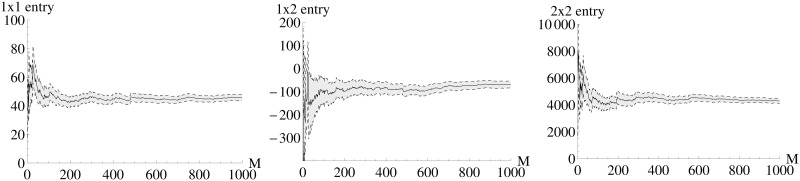
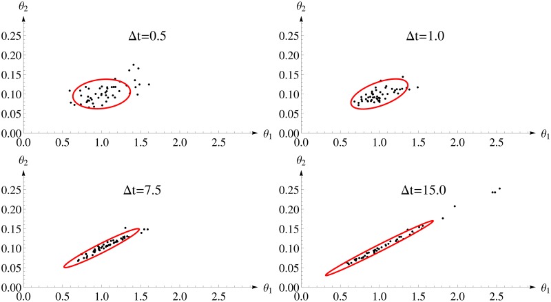
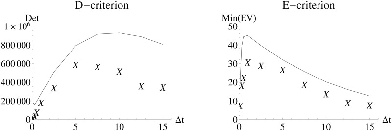
Methods: The Fisher information matrix is the central measure for experimental design as it evaluates the information an experiment provides for parameter estimation. This article suggest an approach to calculate a Fisher information matrix for models containing intrinsic stochasticity and high nonlinearity. The approach makes use of a recently suggested multiple shooting for stochastic systems (MSS) objective function. The Fisher information matrix is calculated by evaluating pseudo data with the MSS technique.

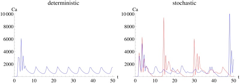
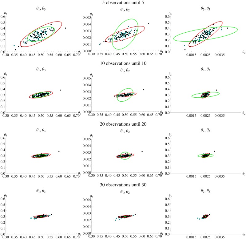
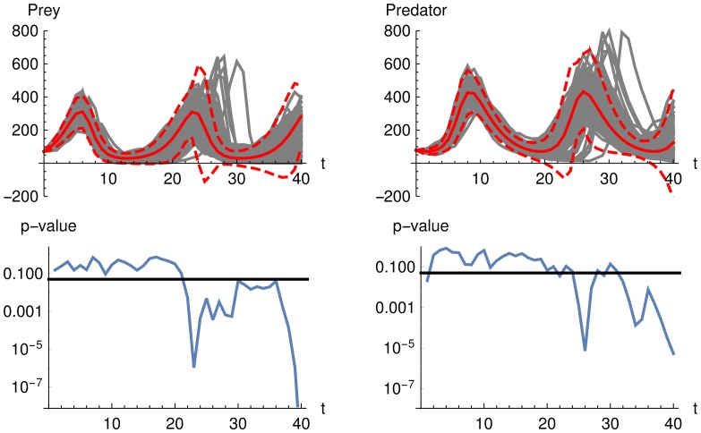
Results: The performance of the approach is evaluated with simulation studies on an Immigration-Death, a Lotka-Volterra, and a Calcium oscillation model. The Calcium oscillation model is a particularly appropriate case study as it contains the challenges inherent to signaling pathways: high nonlinearity, intrinsic stochasticity, a qualitatively different behavior from an ODE solution, and partial observability. The computational speed of the MSS approach for the Fisher information matrix allows for an application in realistic size models.

Fig 1. Deterministic and two (red and blue) stochastic realizations of the Calcium oscillation model.

The left panel shows the deterministic behavior of the Calcium oscillation model, the right panel two stochastic realizations showing the special characteristics to which the experimental design methodology in this article can be applied: qualitatively different behavior from deterministic modeling, bursting oscillations, high nonlinearity and fast dynamics (e.g. from almost 0 to 10000 molecules within a few time units).

Fig 2. Dependence of the accuracy of the FI_MSS entries on the number of pseudo data sets.

Each panel shows one entry of FI_MSS. Note that the 2 × 1 entry is identical to the 1 × 2 entry due to the symmetry of the Fisher information matrix. The x-axis shows the number of pseudo data sets M used for calculating the sample mean (shown as solid line) of Eq 7. Gray color indicates the area from sample mean plus / minus one standard deviation. As the width of the gray are is decreasing, the accuracy increases and an acceptable accuracy is reached at values around M = 200.

Fig 3. Parameter estimates and two dimensional confidence ellipsoids from the FI_MSS Fisher information for different design of the Immigration-Death model.

Each panel considers one experimental design with varying inter-sample distances Δt and 100 observations. The confidence ellipsoid (red) of the FI_MSS is able to represent the shape of the distribution of the estimates.

Fig 4. D-criterion and E-criterion for different experimental designs for the Immigration-Death model.

FI_MSS Fisher information and FI_emp are calculated for different inter-sample distances. The solid line is an interpolation of the values of FI_MSS and the “X” denote the values of FI_emp.

Fig 5. ARSE for different experimental designs for the Immigration-Death model.

FI_MSS and FI_emp are calculated for different inter-sample distances. The solid line is an interpolation of the values of FI_MSS and the “X” denote the values of FI_emp.

Fig 6. Parameter estimates and two dimensional confidence ellipsoids of the benchmark method for different design of the Immigration-Death model.

Each panel considers one experimental design with varying inter-sample distances Δt and 100 observations. The confidence ellipsoid (red) of the FI_Bench corresponds well with the location of the parameter estimates.

Fig 7. D-criterion and E-criterion for different experimental designs for the Immigration-Death model for all three methods (MSS, benchmark and exact).

FI_⋅ Fisher information and FI_emp,⋅ are calculated for different inter-sample distances. The solid line is an interpolation of the values of FI_⋅ and the “x” denote the values of FI_emp,⋅. Red color corresponds to the MSS method, blue to the benchmark and black to the exact method. Symbols partially overlapping.

Fig 8. ARSE for all three method for different experimental designs for the Immigration-Death model.

FI_⋅ and FI_emp,⋅ are calculated for different inter-sample distances. The solid line is an interpolation of the values of FI_ex and the “X” denote the values of FI_emp,⋅. Red color corresponds to the MSS method, blue to the benchmark and black to the exact method. Symbols partially overlapping.

Fig 9. Parameter estimates and two dimensional confidence ellipsoids for the exact method for different design of the Immigration-Death model.

Each panel considers one experimental design with varying inter-sample distances Δt and 100 observations. The confidence ellipsoid (red) of the FI_ex is similar than the confidence ellipsoid of the FI_MSS in Fig 3.

Fig 10. Parameter estimates and confidence ellipsoid from FI_MSS Fisher information for Lotka-Volterra model.

Each row shows one of the scenarios LV1 to LV4. In each row the three panels show one two dimensional projection of the three dimensional parameter space. In each panel the black dots are the estimates from simulated data and the confidence ellipsoid from FI_MSS is marked red.

Fig 11. Dependence of D- and E-criterion on the inter-sample distance.

The left panel shows interpolations of values of the D-criterion and the right panel of the E-criterion for different inter-sample distances.

Fig 12. Parameter estimates and three dimensional confidence ellipsoid from the FI_MSS Fisher information for Lotka-Volterra model.

Left panel fully observed scenario LV1, right panel partially observed scenario LV4. In each panel the black dots are the estimates from simulated data and the three dimensional confidence ellipsoid from FI_MSS is marked yellow. One can see that the FI_MSS Fisher information captures the change in correlation between the parameters.

Fig 13. Parameter estimates and confidence ellipsoid MSS and the benchmark.

Each row shows an experimental design. In each row, each panel shows one two dimensional projection of the three dimensional parameter space. In each graphic the black dots are the estimates from MSS and the green dots from Bench. The confidence ellipsoid of FI_MSS is marked red and the confidence ellipsoid of FI_Bench green. The confidence ellipsoid of FI_Bench for the last row with 30 observations is so small that it can be hardly seen.

Fig 14. Testing the approximation for different observations horizons.

P-values for Kolmogorov-Smirnov tests whether the approximation is fulfilled for different observation horizons; left panel shows results for benchmark and right panel for MSS. Each color stands for one of the 50 data sets. Test is performed with the true parameter θ = (0.5, 0.0025, 0.3).

Fig 15. Mean and two standard deviations from LNA versus stochastic simulations for Lotka-Volterra model.

The upper row shows 100 stochastic simulations in gray color and the mean from a LNA in solid red color as well as mean plus and minus two standard deviations in dashed red color. The lower row shows p-values of a Kolmogorov-Smirnov test for each time point whether the 100 stochastic simulations follow a normal distribution with mean and variance from a LNA. The solid line at a p-value of 0.05 illustrates that all values below show significant differences to the LNA approxiamtion. One can see that the quality of the LNA approximation decreases over time. Test is performed with the parameter θ = (0.5, 0.0025, 0.3).

Fig 16. Dependence of the accuracy of the FI_MSS entries on the number of pseudo data sets.

The x-axis shows the number of pseudo data sets M used for calculating the 2 × 2 entry of FI_MSS, the mean is shown as solid line. Gray color shows the area from sample mean plus / minus one standard deviation. As the width of the gray area is decreasing, the accuracy is increasing. One can see that already small values as M = 400 give a good approximation.

Fig 17. Parameter estimates and confidence ellipsoid from FI_MSS for Calcium model.

The panels show the two dimensional projections of the 12-dimensional parameter space for the Δt = 0.5 design. In each panel the black dots are the estimates from simulated data and the confidence ellipsoid of the Fisher information is marked red. “k” is used as an abbreviation for “thousand”.

Fig 18. Heat map of the difference of correlations between Corr(FI_MSS) and Corr_emp.

A shows the fully observed Calcium oscillation model and B the partially observed scenario. Two correlation matrices are calculated for each of the cases, one from FI_MSS and the other from the estimates. The absolute value of their differences is color-coded.

References

1. Raj A, van Oudenaarden A. Single-Molecule Approaches to Stochastic Gene Expression. Annu Rev Biophys. 2009;38:255–270. 10.1146/annurev.biophys.37.032807.125928 - DOI - PMC - PubMed
1. Gillespie DT. A General Method for Numerically Simulating the Stochastic Time Evolution of coupled Chemical Reactions. Journal of Computational Physics. 1976;22 (4):403–434. 10.1016/0021-9991(76)90041-3 - DOI
1. Pahle J. Biochemical simulations: stochastic, approximate stochastic and hybrid approaches. Briefings in Bioinformatics. 2009;10 (1):53–64. 10.1093/bib/bbn050 - DOI - PMC - PubMed
1. Andreychenko A, Mikeev L, Spieler D, Wolf V. Approximate maximum likelihood estimation for stochastic chemical kinetics. EURASIP Journal on Bioinformatics and Systems Biology. 2012;9. - PMC - PubMed
1. Gillespie CS. Moment-closure approximations for mass-action models. IET Systems Biology. 2009;3 (1):52–58. 10.1049/iet-syb:20070031 - DOI - PubMed
LinkOut - more resources