Space-time codependence of retinal ganglion cells can be explained by novel and separable components of their receptive fields

Abstract

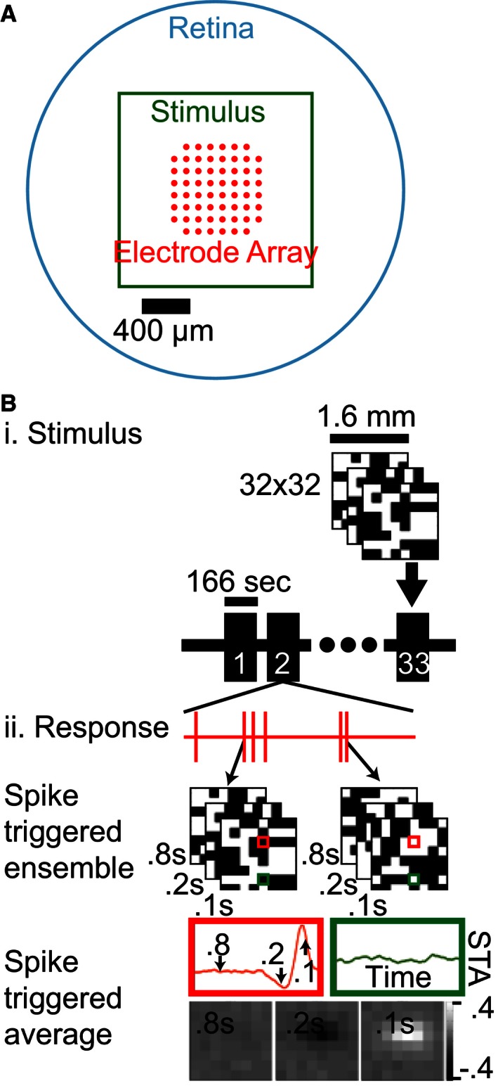
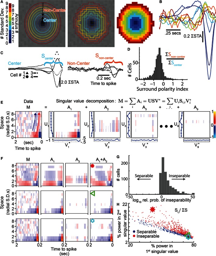
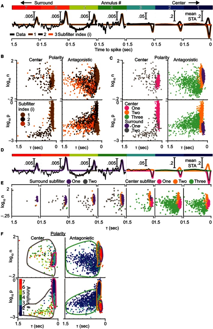
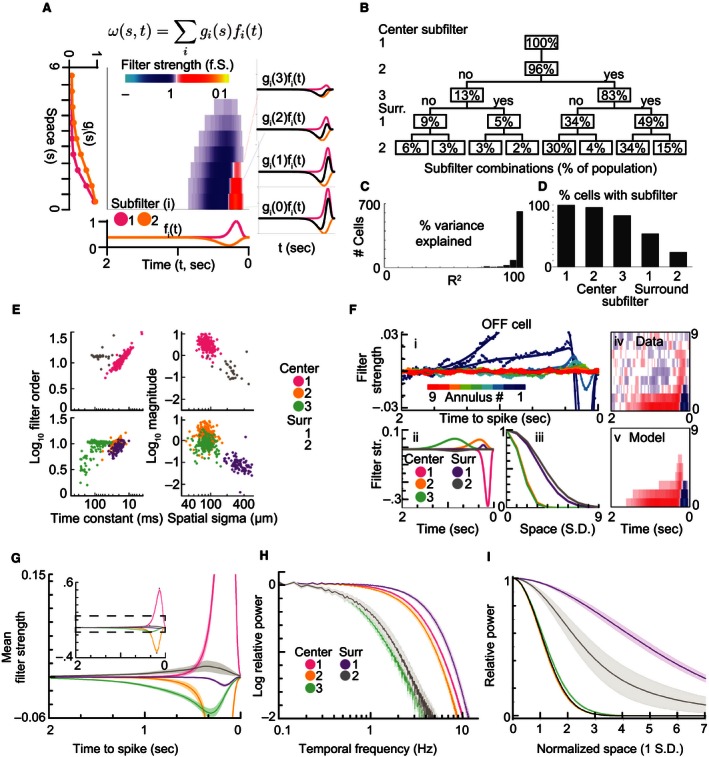
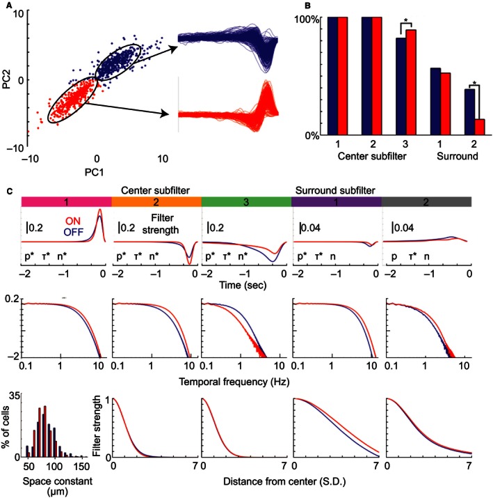
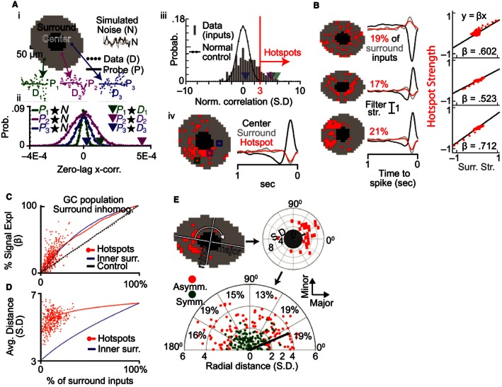
Reverse correlation methods such as spike-triggered averaging consistently identify the spatial center in the linear receptive fields (RFs) of retinal ganglion cells (GCs). However, the spatial antagonistic surround observed in classical experiments has proven more elusive. Tests for the antagonistic surround have heretofore relied on models that make questionable simplifying assumptions such as space-time separability and radial homogeneity/symmetry. We circumvented these, along with other common assumptions, and observed a linear antagonistic surround in 754 of 805 mouse GCs. By characterizing the RF's space-time structure, we found the overall linear RF's inseparability could be accounted for both by tuning differences between the center and surround and differences within the surround. Finally, we applied this approach to characterize spatial asymmetry in the RF surround. These results shed new light on the spatiotemporal organization of GC linear RFs and highlight a major contributor to its inseparability.

Keywords: Retinal ganglion cells; space–time separability; spatiotemporal tuning.

Figure 1

Recording and stimulation of ganglion cells. (A) An explanted mouse retina (cyan) was placed on a multielectrode array (red) ganglion cell side down and stimulated with an optically reduced monitor image (green). (B) i: The stimulus was an iterated sequence of 32 × 32 binary white noise checkerboards (8 × 8 illustrated). ii: Spiking responses of individual cells were identified and used to calculate the average stimulus that triggered a spiking response, the spike‐triggered average (STA). The resulting receptive field map had a space–time structure which can be illustrated as a temporal filter for each spatial point (red and green highlights) or as a spatial filter at a single temporal slice (bottom).

Figure 2

Ganglion cells (GC) linear receptive fields have antagonistic surrounds and many are space–time inseparable. (A) A single Gaussian profile was fit in space–time to localize the receptive field center. Its radial distance isoclines are shown in color for 1σ intervals (left). These annuli are then used to group the spatial inputs into up to nine annular regions (middle and right). (B) Temporal STAs were summated within the annular regions to help determine their dependence on radial distance. (C) To test for a surround, inputs were further grouped into the receptive field center (≤3σ, cyan) and noncenter regions (>3σ, orange) which is illustrated for four example cells. (D) A histogram comparing the first 0.33 seconds of the center (S_center) and noncenter (S_non‐center) responses from all cells, as shown in (C). The predominance of values below zero reveals an antagonistic surround was pervasive in the population. (E) A space–time receptive field map (M, left) that replots the information from (B) into an image using a color map (far right). Singular value decomposition divides the raw STA (M) into nine separable space (U, traces to left of images) and time filters (V, traces below images) that are combined to create the matrices A₁ to A₉. This cell's space–time inseparability can be seen in the spatiotemporal codependence exhibited by the diagonal drift in its raw STA (red and blue arrows) and by the significant power/structure of A₂. (F) The receptive field map (M), first two singular matrices (A₁, A₂), and their sum (A₁+A₂) are shown for three example cells; the top GC (red star) was strongly inseparable, the middle (green triangle) was still inseparable, and the bottom (cyan star) was separable. (G) The relative likelihood of space–time inseparability was higher for the majority of GCs (corrected Akaike information criterion between the A₁ and A₁+A₂ models). (H) Space–time inseparable cells (red, probability of separability < 0.01 from G) had high power in their second singular value compared to the first. Space–time separable cells (blue) had a lower relative power in their second singular value.

Figure 3

Ganglion cell temporal STAs are composed of subfilters with five distinct patterns of spatiotemporal tuning. (A) The average temporal STAs (black traces) within annuli at different radial distances from the receptive field center (see Fig. 2) were each fit by the sum of up to three subfilters (brown/orange traces). Each subfilter is the impulse response of a low‐pass temporal filter. Annular distance is indicated by the primary‐colored bar at the top, with central annuli on the right. (B) Comparison of subfilter properties from all annuli: amplitude (|p|), delay to peak (τ), and filter order (n). Subfilters are divided into center and antagonistic groups based on their polarity relative to the receptive field center. Colors are carried from (A) to illustrate how the subfilter population is obtained. (C) The same plot, recolored into five subfilter types (pastel colors) based on a three‐dimensional (p, τ, n) mixture of Gaussians clustering. Clusters were identified as center or surround based on D and E. (D) The same cell from (A) is shown with its component subfilters colored by the types from (C). Center subfilter types 1 (magenta), 2 (orange), and 3 (green) are located in the central annuli, whereas surround subfilter types 1 (purple) and 2 (gray) are in more distant annuli. (E) The dependence of subfilter type on radial distance is illustrated by breaking plot (C) down by radial distance and combining both polarities. (F) The subfilters from (C) have been recolored by their radial distance from center to demonstrate the dependence of subfilter properties on radial distance. Bordered regions have been added to approximate the boundaries between the subfilter types shown in (C). Within each subfilter type, there is a strong dependence of p on radial distance (vertical rainbow effect in the bottom plots), but no obvious codependence for τ or n. This indicates that individual subfilter types vary their scale but maintain their shape over space, suggesting they are space–time separable.

Figure 4

A model for ganglion cell receptive fields consisting of multiple separable subfilters. (A) The outer products of two pairs (orange and magenta) of spatial g_i(s) and temporal subfilters f_i(t) are summated to generate a space–time inseparable receptive field map. As shown at right, at a given radial distance (s) from the center, the model's temporal filter is the spatially weighted sum (black trace) of the first (magenta trace) and second (orange trace) subfilters. (B) A sequence of F‐tests were used to determine the number of subfilters that were statistically justifiable (P < 0.01 after post hoc correction), the percent of cells reaching each level is visualized. (C) The preferred model explained the majority of the variance in the space–time receptive field. (D) Center subfilters 1, 2, and 3 were present in the majority of cells, whereas surround subfilters 1 and 2 were observed less frequently. (E) i: Models fits (traces) to annular‐averaged STAs (dots) for an example OFF (left) cell. The paired temporal (ii) and spatial (iii) components of the individual subfilters. The space–time codependence in the receptive field map (iv) is accounted for by the model (v). (F) The spatiotemporal properties of the observed subfilters fell into five distinct clusters. Filter time constants are compared to filter order for center polarity (i) and opposite polarity subfilters (ii). Spatial extents are compared to filter magnitude for center polarity (iii) and opposite polarity subfilters (iv). (G) Population average temporal filters from each subfilter type. (H) The same temporal filters averaged in the frequency domain. (I) The average spatial filters for each subtype showed no difference between center subfilters 1, 2, and 3, but surround subfilters 1 and 2 were each significantly different. The first subtype was constrained to a unit normal distribution, and is therefore illustrated in black. Shaded regions in all plots are ±3 SE.

Figure 5

Subfilter properties differ significantly between ON‐ and OFF‐dominated cells. (A) Cells are plotted relative to the first (PC1) and second principal components (PC2) of the temporal STAs at their spatial peak. Two clusters were apparent, the blue group corresponded to OFF‐dominated cells and the red to ON‐dominated cells. (B) Comparison of subfilter observation rates between OFF‐ (blue) and ON‐dominated cells (red). (C) For each subfilter type (columns) we compare the temporal impulse responses (top row), frequency tuning (middle row), and spatial profiles (bottom row) of ON‐ and OFF‐dominated cells. As the first subfilter was constrained to match the original temporal fit, its spatial profile (bottom left) is substituted with the distribution of radial space constants. The asterisk next to p, τ, and n indicates those properties differed significantly between ON‐ and OFF‐dominated cells (P < 0.01, t‐test with post hoc correction).

Figure 6

The receptive field surround contains spatially nonuniform hotspots. (A)i: Raw STA data points (D) are shown for three example inputs in one cell's spatial surround (gray area). The trace through the points is generated using the model fit to the average data (see Fig. 4) and is used as a probe (P) for surround signal in each input. As a control, probes are also compared to simulated STAs that contain only noise (N). Aii: Zero‐lag cross‐correlation is used to compare each probe with the simulated noise, yielding a normal probability distribution unique to each probe (dots and traced distribution) which is used to assess the significance of the probe's correlation with the STA data (arrowheads). Aiii: The data–probe comparisons from (ii) were normalized by the variance of the noise–probe comparisons and the normalized correlations for one cell are binned into this histogram. The observed correlations are positively skewed relative to the unit normal distribution (black trace) that would be expected in the absence of surround signal. Inputs were defined as surround “hotspots” if their normalized cross‐correlation exceeded 3 SD (red vertical line). Aiv: The spatial distribution of surround hotspots (left) and the summed temporal STA in the center (black trace), hotspots (red trace), and surround including hotspots (gray). (B) Example cells with hotspots that were diffusely (top) or densely distributed (middle and bottom) and symmetrical (top and middle) or asymmetrical (bottom). The amount of signal in the surround's summed temporal STA (middle) was estimated by calculating the β between the hotspots and the overall surround strength (right). (C) As a function of the percent inputs in the surround, β between hotspots and the surround was high across the GC population (red dots). The hotspot approach (red trace) outperforms both a random control method (black) and was comparable to selecting the innermost surround inputs first (blue trace). (D) Inputs selected by the hotspot method (red dots) were significantly more distant than when choosing the innermost surround inputs first (blue). (E) Surround asymmetry relative to the major and minor axes of the elliptical receptive field center (top left) was assessed by rotating and normalizing the spatial field of hotspots (top right). The center of mass (black dot and line) of the hotspot inputs (red) is illustrated for an example cell. The bottom polar plot shows that the cell population (n = 256 cells with >=15 hotspot inputs) often had strongly asymmetrical hotspots (red points, sign‐rank test). There was no significant statistical bias in the major or minor axis distribution of the asymmetry. (χ ² test).

References

1. Abd‐El‐Barr, M. M. , Pennesi M. E., Saszik S. M., Barrow A. J., Lem J., Bramblett D. E., et al. 2009. Genetic dissection of rod and cone pathways in the dark‐adapted mouse retina. J. Neurophysiol. 102:1945–1955. - PMC - PubMed
1. Alpern, M. , Fulton A. B., and Baker B. N.. 1987. “Self‐screening” of rhodopsin in rod outer segments. Vision. Res. 27:1459–1470. - PubMed
1. Baden, T. , Berens P., Franke K., Roman Roson M., Bethge M., and Euler T.. 2016. The functional diversity of retinal ganglion cells in the mouse. Nature 529:345–350. - PMC - PubMed
1. Barlow, H. B. 1953. Summation and inhibition in the frog's retina. J. Physiol. 119:69–88. - PMC - PubMed
1. Bloomfield, S. A. 1996. Effect of spike blockade on the receptive‐field size of amacrine and ganglion cells in the rabbit retina. J. Neurophysiol. 75:1878–1893. - PubMed
Publication types
LinkOut - more resources