Pollen dispersal slows geographical range shift and accelerates ecological niche shift under climate change

Abstract

Species may survive climate change by migrating to track favorable climates and/or adapting to different climates. Several quantitative genetics models predict that species escaping extinction will change their geographical distribution while keeping the same ecological niche. We introduce pollen dispersal in these models, which affects gene flow but not directly colonization. We show that plant populations may escape extinction because of both spatial range and ecological niche shifts. Exact analytical formulas predict that increasing pollen dispersal distance slows the expected spatial range shift and accelerates the ecological niche shift. There is an optimal distance of pollen dispersal, which maximizes the sustainable rate of climate change. These conclusions hold in simulations relaxing several strong assumptions of our analytical model. Our results imply that, for plants with long distance of pollen dispersal, models assuming niche conservatism may not accurately predict their future distribution under climate change.

Keywords: adaptation; cline; extinction threshold; gene flow; spatial heterogeneity.

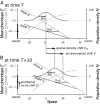
Fig. 1.

Traveling-wave equilibrium (Eq. 6). (A) Scaled population density N (solid black curve), scaled mean phenotype Z (solid black line), and scaled mean growth rate R (solid gray curve; Eq. 5) as a function of space at the traveling-wave equilibrium. The dashed line corresponds to the environmental gradient. The thick segment on the y axis depicts the realized ecological niche. (B) State of the population 10 time units later. Parameters of the dynamic equilibrium are depicted (Eqs. 6–11). Arrows have a length proportional to the rate of the shifts they depict. Parameter values: $A=0.1$, $B=-0.05$, $V=2$, $\gamma =0.65$.

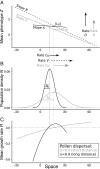
Fig. 2.

Effect of the distance of pollen dispersal (γ, black vs. gray elements) on the properties of the scaled mean phenotype Z (A), of the scaled population density N (B), and of the scaled mean growth rate R (C) at the traveling-wave equilibrium (Eqs. 5–11). The dashed line on A corresponds to the environmental gradient. Arrows have a length proportional to the rates they depict (see text). Parameter values: $A=0.1$, $B=-0.05$, $V=1$.

Fig. 3.

Scaled maximal sustainable rate of the environmental shift for the traveling-wave equilibrium (solid curves, $V_{\text{TW}}^{\text{crit}}$, Eq. 12) and for the uniform-density equilibrium (dashed line, $V_{\text{UD}}^{\text{crit}}$, Eq. 16) as a function of the distance of pollen dispersal (γ), for three values of the slope B of the environmental gradient (A–C). The vertical dotted lines indicate the critical distance of pollen dispersal (${\gamma }_{\text{TW}}^{\text{crit}}$, Eq. 15). Letters E, T, U, and B indicate which equilibrium exists in each part of the parameter space. We used $A=2$. For $B=-1$ (B), the optimal distance of pollen dispersal ${\gamma }_{\text{TW}}^{\text{opt}}$ (Eq. 13) is 0.63 (i.e., $V_{\text{TW}}^{\text{crit}}$ is maximal for $\gamma =0.63$). For $B=-0.4$ (A), ${\gamma }_{\text{TW}}^{\text{opt}}=1$; for $B=-2$ (C), ${\gamma }_{\text{TW}}^{\text{opt}}=0$.

Fig. 4.

Local stability of the equilibria of the three models (A–C), evaluated by numerical resolution (Appendix S1. Numerical Resolution of Eqs. 1 and 3 and Appendix S2. Model with Evolving Genetic Variance). Symbols filling the graphs show the observed equilibria. Lines depict the thresholds $v_{\text{TW}}^{\text{crit}}$, $v_{\text{UD}}^{\text{crit}}$, and ${\gamma }_{\text{TW}}^{\text{crit}}$ using nonscaled variables (Table S1). For the model with evolving genetic variance, we first determined the predicted possible equilibria with the expressions of nonscaled thresholds (Table S1), using the observed value of the genetic variance at the end of the numerical resolution. Then, we determined the observed thresholds $v_{\text{TW}}^{\text{crit}}$, $v_{\text{UD}}^{\text{crit}}$, and ${\gamma }_{\text{TW}}^{\text{crit}}$ as the values of v and γ such that we predict the appropriate switch of equilibria given the observed value of the genetic variance. Parameter values: default parameter values (Table 1) and $r_0=2$ gen.⁻¹. For the model with evolving genetic variance, $v_{\text{LE}}=1$ d². For the two other models, $V_{\text{p}}=2.5$ d² and $V_{\text{g}}=2$ d². Note that with these parameter values, ${\gamma }_{\text{TW}}^{\text{crit}}>0$: the traveling-wave equilibrium therefore does not exist at $\gamma =0$.

Fig. 5.

Features of the traveling-wave equilibrium (A–E) as a function of pollen dispersal distance (γ), using nonscaled variables (Table S1). On C, the dashed horizontal line indicates the speed of environmental change. On E, the dashed horizontal line indicates no ecological niche shift. Parameter values: default parameter values (Table 1) and $r_0=1.5$ gen.⁻¹, $v=11$ km⋅gen.⁻¹. For the model with evolving genetic variance, we used $v_{\text{LE}}=0.05$ d². For the two other models, we used $V_{\text{p}}=0.125$ d² and $V_{\text{g}}=0.1$ d², which is the observed value of the additive genetic variance at equilibrium with the model with evolving genetic variance at $\gamma =0$. The difference between the model with local density dependence (circles) and the model with evolving genetic variance (triangles) therefore depends on the effect of the distance of pollen dispersal on the equilibrium value of the additive genetic variance.

Fig. S1.

Population density n (A, C, and E) and mean phenotype $\overline{z}$ (solid lines in B, D, and F) as a function of space $\zeta =x-vt$ with the simplified model (A and B, $v=32$ km⋅gen.⁻¹) and with the model with local density dependence (C and D: $v=32$ km⋅gen.⁻¹; E and F: $v=45$ km⋅gen.⁻¹) at the traveling-wave equilibrium. The dashed line shows the environmental gradient. The dotted lines show the linear regression weighted by local population size used to estimate the slope s of the realized phenotypic cline. The leading edge corresponds to the right side of each panel. Parameter values: default parameter values (Table 1), and $r_0=2$ gen.⁻¹, $V_{\text{p}}=2.5$ d², $V_{\text{g}}=2$ d², and $\gamma =0.85$. We use here nonscaled parameters (Table S1). The third row (E and F) corresponds to a case close to extinction ($v_{\text{TW}}^{\text{crit}}=46.2$ km⋅gen.⁻¹), and the other rows (A and B, and C and D) show a case far from extinction.

Fig. S2.

Spatial profile at three different times (A and B) and dynamics (C and D) of the genetic variance with the model with evolving genetic variance when the population reaches the traveling-wave equilibrium (A and C) or tends to the uniform-density equilibrium (B and D). The mean genetic variance in C and D is the local genetic variance averaged over space weighted by local population size. Parameter values: default parameter values (Table 1), and $r_0=2$ gen.⁻¹, $v_{\text{LE}}=1$ d². Traveling-wave equilibrium: $v=28.4$ km⋅gen.⁻¹, $\gamma =0.95$; uniform-density equilibrium: $v=14.2$ km⋅gen.⁻¹, $\gamma =0.6$.

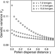
Fig. S3.

Genetic variance at the traveling-wave equilibrium (model with evolving genetic variance) as a function of the distance of pollen dispersal γ for three rates of the environmental shift. Parameter values: default parameter values (Table 1), and $r_0=1.5$ gen.⁻¹, $v_{\text{LE}}=0.05$ d².

References

1. Parmesan C. Ecological and evolutionary responses to recent climate change. Annu Rev Ecol Evol Syst. 2006;37(1):637–669.
1. Selwood KE, McGeoch MA, Mac-Nally R. The effects of climate change and land-use change on demographic rates and population viability. Biol Rev Camb Philos Soc. 2015;90(3):837–853. - PubMed
1. Urban MC. Accelerating extinction risk from climate change. Nature. 2015;348(6234):571–573. - PubMed
1. Davis MB, Shaw RG, Etterson JR. Evolutionary responses to changing climate. Ecology. 2005;86(7):1704–1714.
1. Bellard C, Bertelsmeier C, Leadley P, Thuiller W, Courchamp F. Impacts of climate change on the future of biodiversity. Ecol Lett. 2012;15(4):365–377. - PMC - PubMed
Publication types
LinkOut - more resources