Evolutionary learning of adaptation to varying environments through a transgenerational feedback

Abstract

Organisms can adapt to a randomly varying environment by creating phenotypic diversity in their population, a phenomenon often referred to as "bet hedging." The favorable level of phenotypic diversity depends on the statistics of environmental variations over timescales of many generations. Could organisms gather such long-term environmental information to adjust their phenotypic diversity? We show that this process can be achieved through a simple and general learning mechanism based on a transgenerational feedback: The phenotype of the parent is progressively reinforced in the distribution of phenotypes among the offspring. The molecular basis of this learning mechanism could be searched for in model organisms showing epigenetic inheritance.

Keywords: bet hedging; environmental fluctuations; epigenetic inheritance; evolution; population growth.

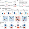
Fig. 1.

Schematic view of the evolutionary learning mechanism. (A) Each individual (solid circle) randomly expresses a phenotype ${\varphi }_{\text{A}}$ (blue) or ${\varphi }_{\text{B}}$ (red) according to a probability distribution ${\pi }_i$ $\left(i=\mathrm{A},\mathrm{B}\right).$ In an environment ${\epsilon }_j$ $(j=\mathrm{A},\mathrm{B};$ background colors), a phenotype ${\varphi }_i$ has a fitness value $w_i^{\left(j\right)}.$ Under extreme selection, only individuals whose phenotype matches the environment survive and produce offspring; individuals with mismatched phenotypes die (crossed out). (B) The learning rule: Each individual in a new generation $t+1$ inherits a probability ${\pi }_i\left(t+1\right)$ that equals the probability ${\pi }_i\left(t\right)$ carried by its parent plus a change $\mathrm{\Delta }{\pi }_i$ that depends on the parent phenotype. This change makes the offspring more likely $\left(\mathrm{\Delta }{\pi }_i>0\right)$ to have the same phenotype as the parent and less likely $\left(\mathrm{\Delta }{\pi }_i<0\right)$ otherwise. (C) Evolutionary learning in a varying environment: Bar plots show the phenotype probability distributions ${\pi }_i\left(t\right)$ in each generation. After a few generations, ${\pi }_i\left(t\right)$ approaches the environment frequencies as a result of the learning mechanism. (D) Lineages of individuals: Solid arrows form a continuous lineage; dashed arrows are where a lineage terminates. The history of phenotypes along a continuing lineage reflects the past environment.

Fig. S1.

Asymptotic growth rate $\mathrm{\Lambda }$ as a function of the learning rate η for given patterns of environmental variations, assuming two possible environments, ${\epsilon }_{\text{A}}$ and ${\epsilon }_{\text{B}},$ and extreme selection. The constant term, ${\mathrm{\Lambda }}_{\mathrm{s}},$ is the asymptotic growth rate that would be achieved by perfect sensing with no cost. (A–C) Periodic environmental changes with fixed durations ${\tau }_{\text{A}}$ and ${\tau }_{\text{B}}$ for each environment, respectively, where ${\tau }_{\text{A}}={\tau }_{\text{B}}=5$ (A), 10 (B), and 40 (C). (D–F) Environmental durations are geometrically distributed with means equal to ${\tau }_{\text{A}}$ and ${\tau }_{\text{B}},$ respectively, where ${\tau }_{\text{A}}=10/3,{\tau }_{\text{B}}=10/7$ (D); ${\tau }_{\text{A}}={\tau }_{\text{B}}=3$ (E); and ${\tau }_{\text{A}}={\tau }_{\text{B}}=10$ (F).

Fig. S2.

Adaptation timescale ${\tau }_{\text{ad}}^{*}$ corresponding to the optimal learning rate $\eta \ast ,$ for different patterns of environmental variations as shown in Fig. S1. (A) Periodic environmental changes with a fixed duration ${\tau }_{\text{env}}.$ (B) Geometrically distributed environmental durations with a same mean equal to ${\tau }_{\text{env}}.$ Error bars are due to uncertainty in numerical calculations. Dashed lines represent critical values of ${\tau }_{\text{env}}$ below which $\eta \ast \to 0,$ and hence ${\tau }_{\text{ad}}^{*}\to \mathrm{\infty }\mathrm{.}$

Fig. S3.

Simulation of population growth with different learning rates, under nonextreme selection with given patterns of environmental variations. The fitness matrix is chosen to be the same as in Fig. 2 of the main text; i.e., $w_i^{\hspace{0.17em}\left(j\right)}=\left[\left[2.0,0.2\right],\left[0.2,2.0\right]\right].$ Colored lines represent learning rates ranging from $\eta =0.05$ to 0.30. (A) Environment is i.i.d. $\left({\tau }_{\text{env}}\simeq 1\right)$ with probabilities $p_{\text{A}}=0.7$ and $p_{\text{B}}=0.3,$ as in Fig. 2C. The population adopts bet-hedging behavior. (B) Environmental durations are geometrically distributed with the mean ${\tau }_{\text{env}}=10.$ Shaded regions mark intermittent periods of time during which the population shows transgenerational plasticity, whereas in open regions the population behaves more similarly to bet hedging. (C) Environment switches periodically between two conditions every ${\tau }_{\text{env}}=40$ generations, as in Fig. 2D. The population shows transgenerational plasticity. (D) The pattern of environmental variations alternates every 200 generations between being i.i.d. $({\tau }_{\text{env}}\simeq 1,$ as in A) and periodic $({\tau }_{\text{env}}=40,$ as in C). The population exhibits either bet hedging or transgenerational plasticity during the corresponding periods of time.

Fig. 2.

Simulation of a learning population in a fluctuating environment. The environment alternates between two conditions ${\epsilon }_{\text{A}}$ and ${\epsilon }_{\text{B}}.$ Each individual carries a probability distribution $({\pi }_{\text{A}},$ ${\pi }_{\text{B}})$ and randomly selects a phenotype ${\varphi }_{\text{A}}$ or ${\varphi }_{\text{B}}.$ Each phenotype ${\varphi }_i$ has a fitness $w_i^{\hspace{0.17em}\left(j\right)}$ in the environment ${\epsilon }_j,$ where $w_i^{\hspace{0.17em}\left(j\right)}=\left[\left[2.0,0.2\right],\left[0.2,2.0\right]\right].$ The learning rate is $\eta =0.1,$ which corresponds to ${\tau }_{\text{ad}}\approx 10.$ (A–C) Blue shades represent the histograms of the probability ${\pi }_{\text{A}}\left(t\right)$ in each generation t estimated from $N={10}^5$ individuals, with normally distributed initial values ${\pi }_{\text{A}}\left(0\right)\sim \mathcal{N}\left(0.5,0.05\right);$ yellow lines are the average probability ${\overline{\pi }}_{\text{A}}\left(t\right)$ over the population. (D–F) Blue lines are the population growth curves estimated from the ${\pi }_{\text{A}}\left(t\right)\text{s}$ in the same examples as in A–C; black lines represent the optimal bet-hedging solutions calculated from the environment frequencies; yellow lines are the maximum growth curve obtained by having the phenotype matching the environment at all times and with no cost for sensing. (A and D) The environment is independent and identically distributed $\left({\tau }_{\text{env}}\simeq 1\right)$ with $p_{\text{A}}=0.7,$ $p_{\text{B}}=0.3.$ (B and E) The durations of the environment ${\epsilon }_{\text{A}}$ and ${\epsilon }_{\text{B}}$ are geometrically distributed with means ${\tau }_{\text{A}}=10$ and ${\tau }_{\text{B}}=5,$ respectively. (C and F) The environment switches every ${\tau }_{\text{env}}=40$ generations.

References

1. Lambert G, Kussell E. Memory and fitness optimization of bacteria under fluctuating environments. PLoS Genet. 2014;10(9):e1004556. - PMC - PubMed
1. Amasino R. Seasonal and developmental timing of flowering. Plant J. 2010;61(6):1001–1013. - PubMed
1. Slatkin M. Hedging one’s evolutionary bets. Nature. 1974;250(5469):704–705.
1. Philippi T, Seger J. Hedging one’s evolutionary bets, revisited. Trends Ecol Evol. 1989;4(2):41–44. - PubMed
1. Simons AM. Modes of response to environmental change and the elusive empirical evidence for bet hedging. Proc R Soc B. 2011;278(1712):1601–1609. - PMC - PubMed
Publication types
LinkOut - more resources