A 2D virtual reality system for visual goal-driven navigation in zebrafish larvae

Abstract

Animals continuously rely on sensory feedback to adjust motor commands. In order to study the role of visual feedback in goal-driven navigation, we developed a 2D visual virtual reality system for zebrafish larvae. The visual feedback can be set to be similar to what the animal experiences in natural conditions. Alternatively, modification of the visual feedback can be used to study how the brain adapts to perturbations. For this purpose, we first generated a library of free-swimming behaviors from which we learned the relationship between the trajectory of the larva and the shape of its tail. Then, we used this technique to infer the intended displacements of head-fixed larvae, and updated the visual environment accordingly. Under these conditions, larvae were capable of aligning and swimming in the direction of a whole-field moving stimulus and produced the fine changes in orientation and position required to capture virtual prey. We demonstrate the sensitivity of larvae to visual feedback by updating the visual world in real-time or only at the end of the discrete swimming episodes. This visual feedback perturbation caused impaired performance of prey-capture behavior, suggesting that larvae rely on continuous visual feedback during swimming.

Figure 1. Quantification of tail movements in free-swimming conditions.

Row depict movements from different categories. (a) Superimposition of the image of a larva during a tail bout. The first image is in light blue and successive images are darker. The path followed by the head is shown by a red line, the black arrows represent the head orientation at the beginning and end of the bout. (b) Illustration of the image processing method to a characteristic snapshot of the movement in (a), an ellipse was fitted on the binarized image of the larva (in black). Pixels were split in two groups according to the major axis of the black ellipse: pixels shown in red or blue, superimposed on the larva. For each of these two groups of pixels, a second ellipse was fitted (red and blue ellipse) and the corresponding minor axes were drawn in red and blue. The center of curvature (black dot) was defined as the intersection between the two minor axes. The deflection was defined as the inverse of the average distance between all the pixels in the larva and the center of the curvature (1/R). To obtain a dimensionless value, the result was multiplied by the length of the larva at rest L_o. The sign of the deflection was computed as left = negative and right = positive. (c) The resulting deflection of the tail over time, for each of the different types of movements in (a).

Figure 2. Prediction of the larva’s trajectory from the deflection of the tail.

(a) Parametrization of the displacement of the larva in the horizontal plane. Only 3 parameters are required to describe the trajectory: the axial, lateral and yaw speed. (b) Illustration of the Auto-regressive Model with External Input. Each of the three parameters of trajectory was computed using the tail deflection. 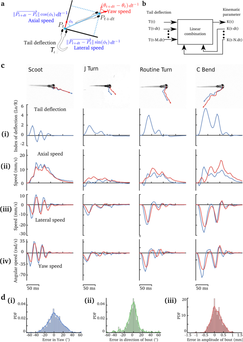Each of the kinematic parameters at time t, K(t) was computed using a linear combination of its past values: and the present and past values of the tail deflection: . 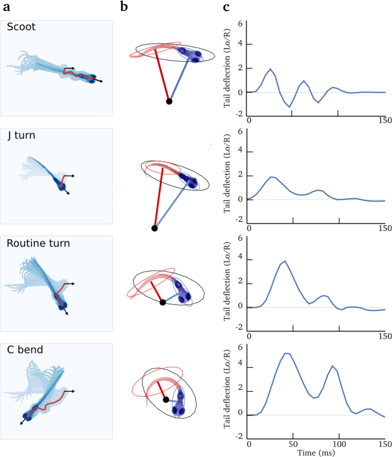See Materials and Methods for details. (c) Examples of four different types of movements showing the true path of the larva (in blue) and that predicted (in red). (i) Tail deflection corresponding to different categories of movement. (ii) The axial speed. (iii) The lateral speed. (iv) Yaw angle. For each case, the observed kinematic parameter is in red, and the predicted in blue. (d) Distribution of the errors between the predicted position and orientation, and those observed, for: (i) change in head orientation; (ii) direction of movement; (iii) amplitude of the tail bout. The results presented in (c) and (d) were taken from the test dataset.

Figure 3. The optomotor response in virtual reality.

(a) A schematic of the experimental setup. The tail was imaged using a high-speed camera, an IR LED for illumination, and a high-pass filter to prevent the visual stimulus from reaching the camera. A projector was used to display the moving grating on a diffusive screen placed 0.5 cm below the larva. The larva was head-embedded in low-melting agarose at the bottom of a petri-dish. The tail was free to move. (b) The grating moved at 1 cm/s. θ represents the difference between the larva’s heading direction (green arrow) and the direction of the moving grating (yellow arrow). (c) Center panel: example of the changes in θ for one larva (20 trials). Left panel: Initial distribution of θ for the same larva. Right panel: Final orientation (θ_t=6s) distribution. The initial orientation distribution (θ_t=0) is superimposed in blue for comparison. (d) Left panel: Initial orientation distribution for all larvae and all trials for which at least one bout was generated. Center panel: color-coded density of trajectory as a function of time for the 6 s trials. Left panel: Initial distribution of θ_t=0 for all larvae. Right panel: Final orientation distribution (θ_t=6s) for all larvae. 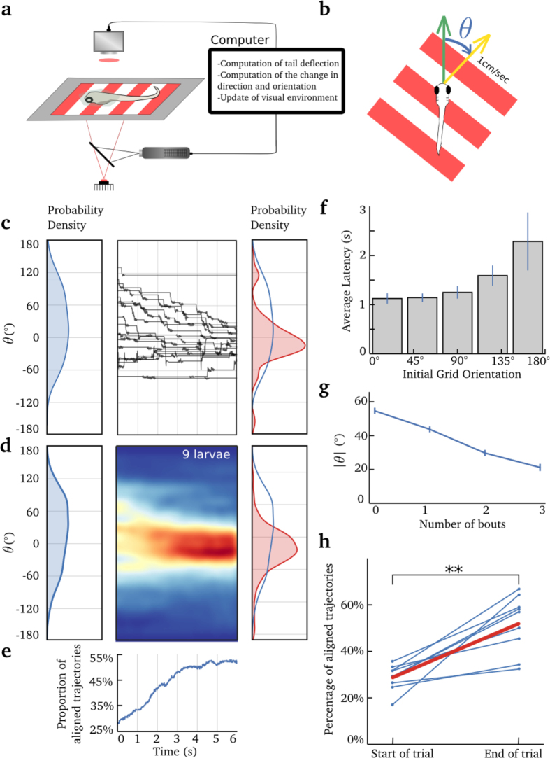(e) Proportion of larvae aligned with the moving stimuli () as a function of time during the trial. The time scale is common to (c), (d) and (e). (f) Histogram of latency as a function of the initial orientation of the grating, error bar indicates s.e.m. (g) Average of |θ|, for successive bouts, error bar indicates s.e.m. (h) Average percentage of trajectories aligned with the moving stimulus (), at the beginning and at the end of the trials, for each larva. The average is shown in red.

Figure 4. Prey-capture behavior in virtual reality.

(a) Schematic of the experimental setup. The larva is positioned on an elevated stage in the center of a cylindrical recording chamber. Visual stimuli were projected on a screen surrounding the recording chamber, covering a field of view of 180°, and centered around the direction of the larva’s head. The tail was imaged using a high-speed camera mounted on a binocular. For illumination, an IR LED was placed below the chamber. Two projectors were used to project the virtual prey, each covering a field of view of 90°. (b) Presentation of the virtual environment during each trial. (i) The virtual prey of 4° appeared from either side of the larva with an angular speed of 20°/s. (ii) After the onset of the first tail bout, the angular speed of the virtual prey was set to 0°/s and its position on the screen was further updated according to the larva’s tail movements only. (iii) A trial was considered successful if the larva got at least 400 μm from the virtual prey. (c) Percentage of trials that ended in successful capture of the virtual prey. Only trials where larvae executed at least one tail bout were considered. Left: Each dot represents the performance of individual larvae. Right: The performance obtained by shuffling the angular positions of the virtual prey in each dataset. The red segment depicts the average. (p = 1.4*10⁻⁵, Wilcoxon signed-rank test). (d) Examples of paths of a larva towards the virtual prey. The paths are color-coded according to the position of the virtual prey at the onset of the first tail bout (color bar). Upper panel: Individual paths for one larva. Left: Paths leading to capture. Right: paths failing to capture the virtual prey. Lower panel: Superposition of the trajectories from all larvae (N = 27). Each bin of the meshgrid is color-coded according to the average position of the virtual prey for the trajectory in that bin (color bar). Left: paths leading to capture. Right: Paths failing to capture the virtual preys. In all panels, the black arrows indicate the initial position of larvae. (e) Distribution of the angle of the virtual prey at the bout’s onset in the first trial. (f) Proportion of bouts in each category of movement, during the trials (virtual-prey stimuli) and between trials (spontaneous). Not Significant: *p > 0.05, p < 0.05, **p < 0.01, ***p < 0,001. (g) Proportion of bouts in each category of movement for successful or unsuccessful trials. (h) Change in head orientation for the first three bouts. Only trials in which larvae performed at least three bouts were considered. Error bar: s.e.m.

Figure 5. Delayed visual feedback affects prey-capture behavior.

(a) Tail deflection of the larva and the corresponding modification of the virtual-prey position (visual feedback): angular position and size of the virtual prey. Left panel: feedback was continuously updated during tail movements (green). Right panel: the feedback was delayed and presented only after the end of the bout (the time indicated by the vertical dashed lines). The green segments on all curves indicate the detection of tail bouts and the corresponding modification in size and position of the virtual prey. (b) Average duration of bouts in real-time and delayed feedback conditions, for each larva. The average is shown in red. (p = 0.0012, Wilcoxon signed-rank test). (c) Normalized bouts: the paths of each bout was rotated and rescaled according to the position of the virtual prey (black dot). The starting position is indicated by the black cross. Upper panel: normalized bouts for all larvae when the feedback was presented in real time. Middle panel: normalized bouts of all larvae, when the feedback was presented at the end of a bout (delayed feedback). Lower panel: ratio of the density of normalized bouts. The color bar indicates the ratio of density between the real-time and delayed feedback conditions (>1 indicates that the density of paths is larger for the real-time with respect to the delayed feedback) (d) Cumulative distribution of the normalized distance to the virtual prey at the end each bout, for trials in which the feedback was provided in real time (blue) or after the end of the bout (red). The distribution were significantly different (p = 0.04, Kolmogorov-Smirnov test). A normalized distance of 0.5 means that the bouts reduced the distance to the prey by half. (e) Percentage of trials that ended in a successful capture of the virtual prey, for real-time feedback (left), and delayed feedback trials (right) (from 27 larvae). The red segment depicts the average.

References

1. Edelman S. The minority report: some common assumptions to reconsider in the modelling of the brain and behaviour. Journal of Experimental & Theoretical Artificial Intelligence 28, 1–26 (2015).
1. Chen X. & Engert F. Navigational strategies underlying phototaxis in larval zebrafish. Front. Syst. Neurosci. 8 (2014). http://dx.doi.org/10.3389/fnsys.2014.00039. - DOI - PMC - PubMed
1. Mischiati M. et al. Internal models direct dragonfly interception steering. Nature 517, 333–338 (2015). - PubMed
1. Ofstad T. A., Zuker C. S. & Reiser M. B. Visual place learning in drosophila melanogaster. Nature 474, 204–207 (2011). - PMC - PubMed
1. Aronov D. & Tank D. W. Engagement of neural circuits underlying 2d spatial navigation in a rodent virtual reality system. Neuron 84, 442–456 (2014). - PMC - PubMed
LinkOut - more resources