Smooth versus Textured Surfaces: Feature-Based Category Selectivity in Human Visual Cortex

Abstract

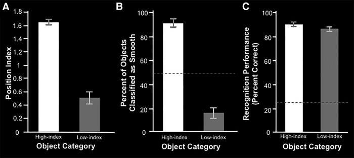
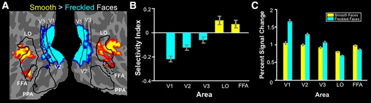
In fMRI studies, human lateral occipital (LO) cortex is thought to respond selectively to images of objects, compared with nonobjects. However, it remains unresolved whether all objects evoke equivalent levels of activity in LO, and, if not, which image features produce stronger activation. Here, we used an unbiased parametric texture model to predict preferred versus nonpreferred stimuli in LO. Observation and psychophysical results showed that predicted preferred stimuli (both objects and nonobjects) had smooth (rather than textured) surfaces. These predictions were confirmed using fMRI, for objects and nonobjects. Similar preferences were also found in the fusiform face area (FFA). Consistent with this: (1) FFA and LO responded more strongly to nonfreckled (smooth) faces, compared with otherwise identical freckled (textured) faces; and (2) strong functional connections were found between LO and FFA. Thus, LO and FFA may be part of an information-processing stream distinguished by feature-based category selectivity (smooth > textured).

Keywords: FFA; LO; fMRI; functional connectivity; texture.

Figure 1.

Sample images of objects used to generate synthetic stimuli and resultant stimuli. A, Left, Intact object stimuli used for the imaging and psychophysics experiments (Experiments 1a and 1b), and to generate the TS stimuli. Right, Scrambled object stimuli used to generate the TS− set of stimuli. B, Sample synthetic stimuli used for the imaging and psychophysics experiments (Experiments 1a and 1b). Left, TS stimuli. Right, TS− stimuli.

Figure 2.

Schematic depiction of the method used to rank 300 objects based on their image statistics. The two-parameter case is depicted for ease of visualization (2457 parameters actually used). A, Image properties of 16 intact objects were measured (unfilled cyan circles). The mean of each parameter was then computed to arrive at the mean “location” for intact objects (filled cyan circle). The same procedure was repeated for the images of scrambled objects (purple circle in B). B, The vector pointing from the scrambled objects to the intact objects in the parameter space was obtained by taking the difference between these two points. C, Subtracting the obtained difference from all points defines a new vector space, with the scrambled objects point at the origin (position = 0). Normalization places the intact objects point at unit length (position = 1). For each of 300 independent objects (unfilled gray circle), image properties were measured and represented as a point in this parameter space. This point was then projected onto the intact–scrambled object axis. The position along this axis denotes the level of similarity between a given object and the scrambled objects image set.

Figure 3.

All stimuli from the high-index (smooth) and low-index (textured) stimuli sets used in Experiments 2b and 2c.

Figure 4.

Mean position index for the stimulus sets used in Experiments 1, 2, and 3. Intact objects and scrambled objects sets were used to define the intact–scrambled axis and also served to create the TS and TS− stimuli used in Experiment 1, respectively.

Figure 5.

LO localizer stimuli and results for subjects in Experiment 1. A, Examples of stimuli used to localize LO for all subjects. Left, Intact object stimuli. Right, Grid-scrambled object stimuli. B, Left, Lateral view of both hemispheres of a group average activity map, based on fixed-effect analysis, in surface-inflated format showing the response to intact vs scrambled objects for 10 subjects. Right, The same group average map in a flattened surface format. Absolute threshold range. 10⁻¹⁶ to 10⁻³². Borders of LO and other regions of interest are delineated with black lines. The asterisk marks the location of the foveal representation. Light gray denotes gyri, and dark gray denotes sulci.

Figure 6.

Behavioral and imaging results for Experiment 1. A, Mean recognition performance ± SEM for five subjects in a four-alternative forced-choice task. Dashed line indicates chance performance (25%). B, ROI results from the same group of subjects shown in Figure 1B (n = 10) shown as the mean of the selectivity index ± SEM for the TS over the TS− condition. C, Percentage signal change from baseline for intact objects, TS stimuli, and TS− stimuli separately. Blue bars indicate ROIs for which the response to TS stimuli is significantly lower than the response to TS− stimuli. Yellow bars indicate the opposite effect. See Table 3 for raw values for each hemisphere.

Figure 7.

Computational results for Experiment 2a and behavioral results for Experiment 2b. A, Mean position index ± SEM for the top 16 (high-index/smooth) and bottom 16 (low-index/textured) objects. B, Visual appearance classification performance ± SEM for five subjects in a two alternative forced-choice task (smooth or textured). Data are shown as the mean percentage of trials in which subjects classified the objects as smooth. The dashed line indicates chance performance (50%). C, Mean recognition performance ± SEM for five subjects in a four-alternative forced-choice task. Dashed line indicates chance performance (25%).

Figure 8.

fMRI results from Experiment 2c. A, Flattened-surface format for both hemispheres of a group average map, based on fixed effect analysis showing the response to intact versus scrambled objects for 12 subjects. Absolute threshold range: 10⁻³⁰ – 10⁻⁵⁰. Other conventions are as in Figure 1B. B, Flattened-surface format for both hemispheres of a group average map, based on random-effects analysis, showing the response to smooth vs textured (high-index vs low-index) objects for the same 12 subjects. Absolute threshold range, 0.05 to 10⁻³. C, ROI results for the same 12 subjects shown as the mean of the selectivity index ± SEM for the smooth over textured objects. D, Percentage signal change from baseline for smooth and textured objects, separately. Blue bars indicate ROIs for which the response to smooth objects is significantly lower than the response to textured objects. Yellow bars indicate the opposite preference. Error bars indicate SEM. See Table 4 for raw values for each hemisphere.

Figure 9.

Stimuli from Experiment 3. A, Sample stimuli used in Experiment 3. Top, Computer-generated faces with smooth complexion. Bottom, Same computer-generated faces with freckles. B, Mean position index ± SEM for the smooth and freckled faces used in Experiment 3.

Figure 10.

Results from Experiment 3. A, Flattened-surface format of both hemispheres of a group average map, based on random-effects analysis, showing the response to smooth vs freckled faces for 15 subjects. Absolute threshold range, 0.05 to 10⁻³. Other conventions are as in Figure 1B. B, ROI results for the same 15 subjects shown as the mean of the selectivity index ± SEM for the smooth over freckled faces. C, Percentage signal change from baseline for smooth and freckled faces, separately. Blue bars indicate ROIs for which the response to smooth faces is significantly lower than the response to freckled faces. Yellow bars indicate the opposite effect. See Table 5 for raw values for each hemisphere.

Figure 11.

Functional connectivity analysis methods and results from Experiment 4. A, Possible organization for LO and FFA with V3 as a common input. B, C, Alternative possibilities for a hierarchical architecture between LO and FFA. D, Hybrid alternative. E, Flattened-view format of the right hemisphere of a common surface showing the regions of the cortex used as both seeds and sampling ROIs. F, Mean correlation ± SEM within each of the sampled ROIs for the different seeding configurations for 29 subjects.

References

1. Aguirre GK, Detre JA, Alsop DC, D'Esposito M (1996) The parahippocampus subserves topographical learning in man. Cereb Cortex 6:823–829. - PubMed
1. Albright TD (1984) Direction and orientation selectivity of neurons in visual area MT of the macaque. J Neurophysiol 52:1106–1130. - PubMed
1. Balas BJ (2006) Texture synthesis and perception: using computational models to study texture representations in the human visual system. Vision Res 46:299–309. 10.1016/j.visres.2005.04.013 - DOI - PubMed
1. Brainard DH (1997) The psychophysics toolbox. Spat Vis 10:433–436. - PubMed
1. Brodeur MB, Dionne-Dostie E, Montreuil T, Lepage M (2010) The Bank of Standardized Stimuli (BOSS), a new set of 480 normative photos of objects to be used as visual stimuli in cognitive research. PLoS One 5:e10773 10.1371/journal.pone.0010773 - DOI - PMC - PubMed
LinkOut - more resources