Explaining Support Vector Machines: A Color Based Nomogram

Abstract

Problem setting: Support vector machines (SVMs) are very popular tools for classification, regression and other problems. Due to the large choice of kernels they can be applied with, a large variety of data can be analysed using these tools. Machine learning thanks its popularity to the good performance of the resulting models. However, interpreting the models is far from obvious, especially when non-linear kernels are used. Hence, the methods are used as black boxes. As a consequence, the use of SVMs is less supported in areas where interpretability is important and where people are held responsible for the decisions made by models.

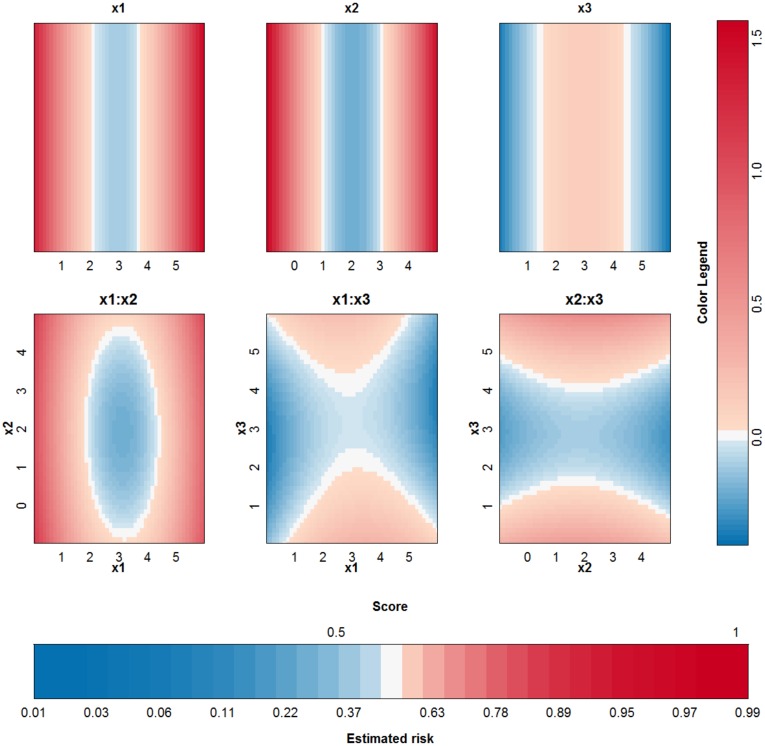
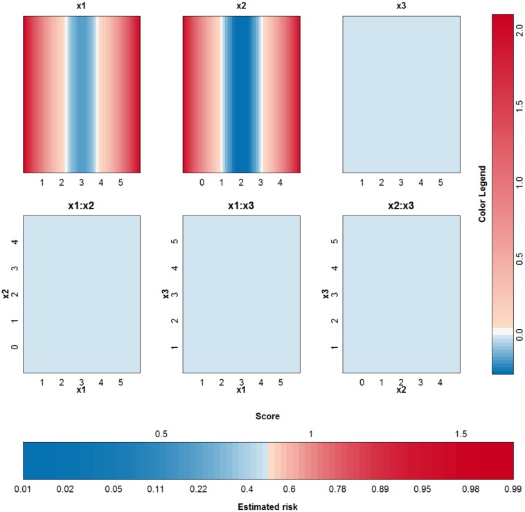
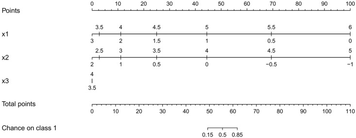
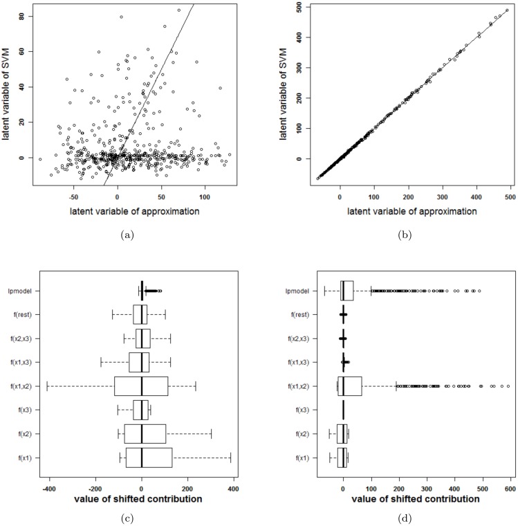
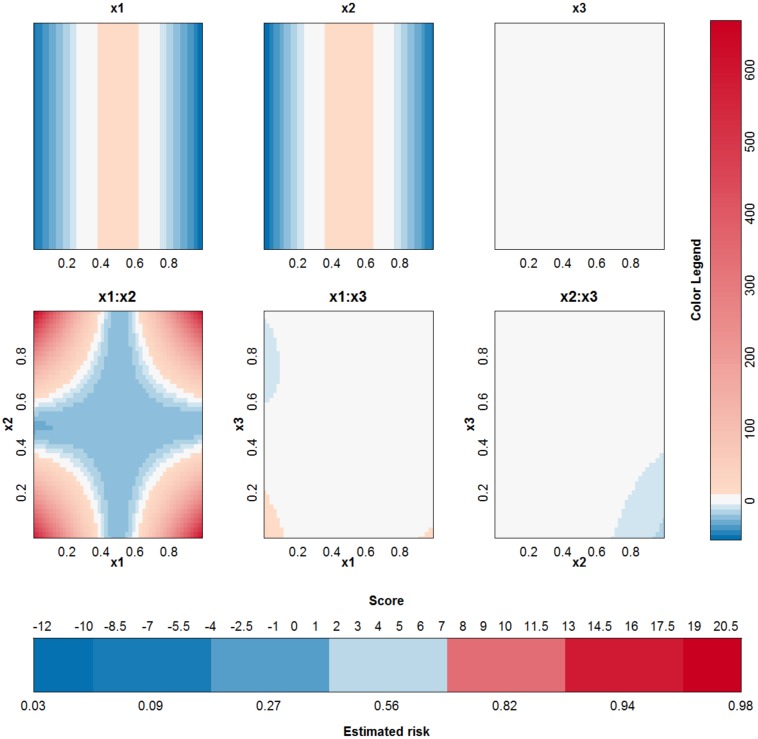
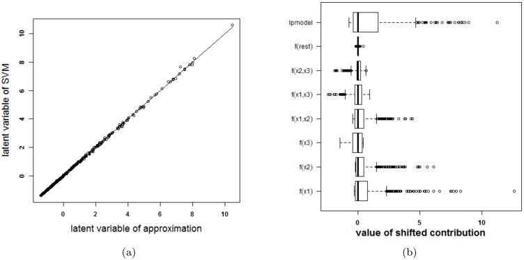
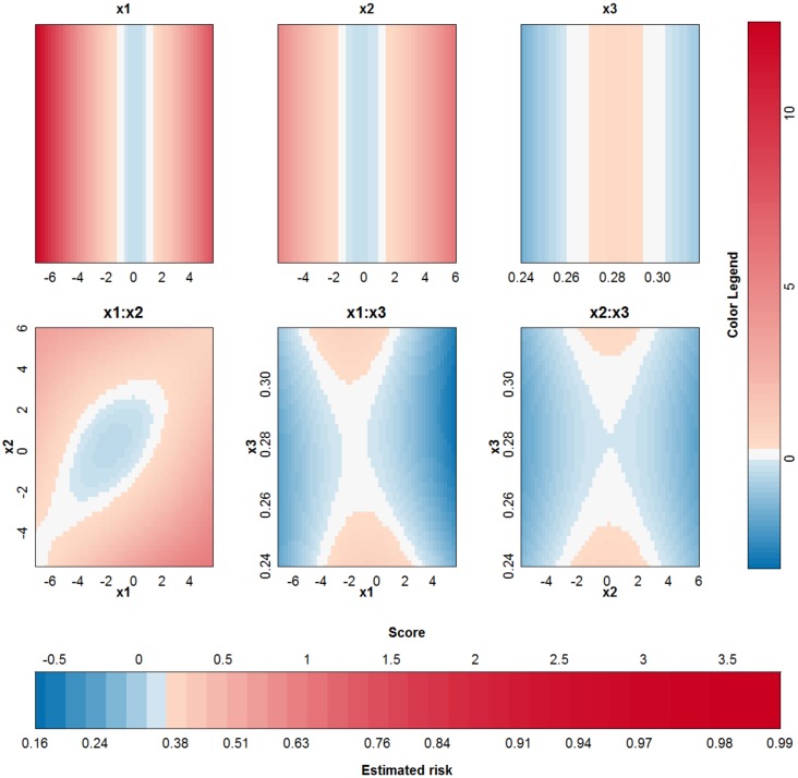
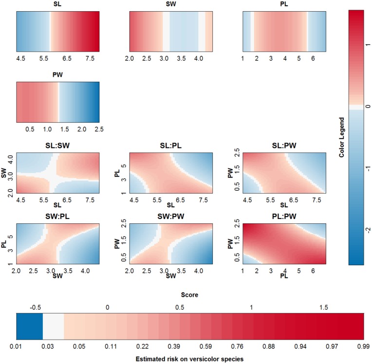
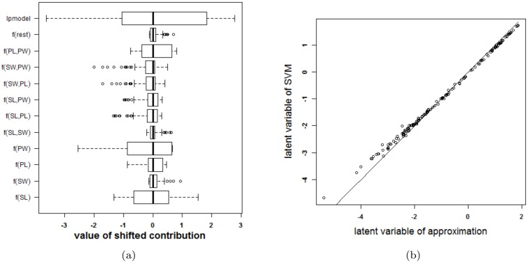
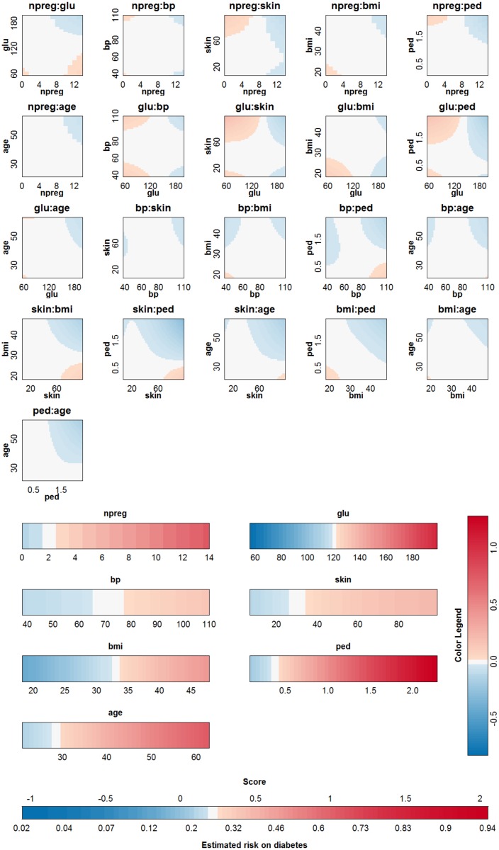
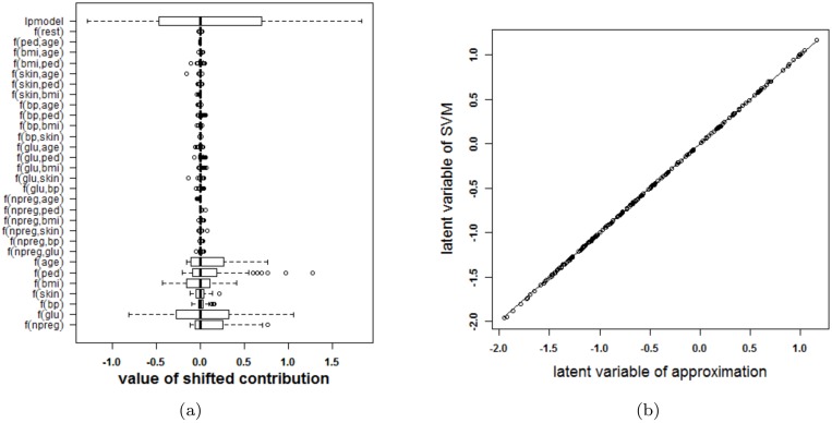
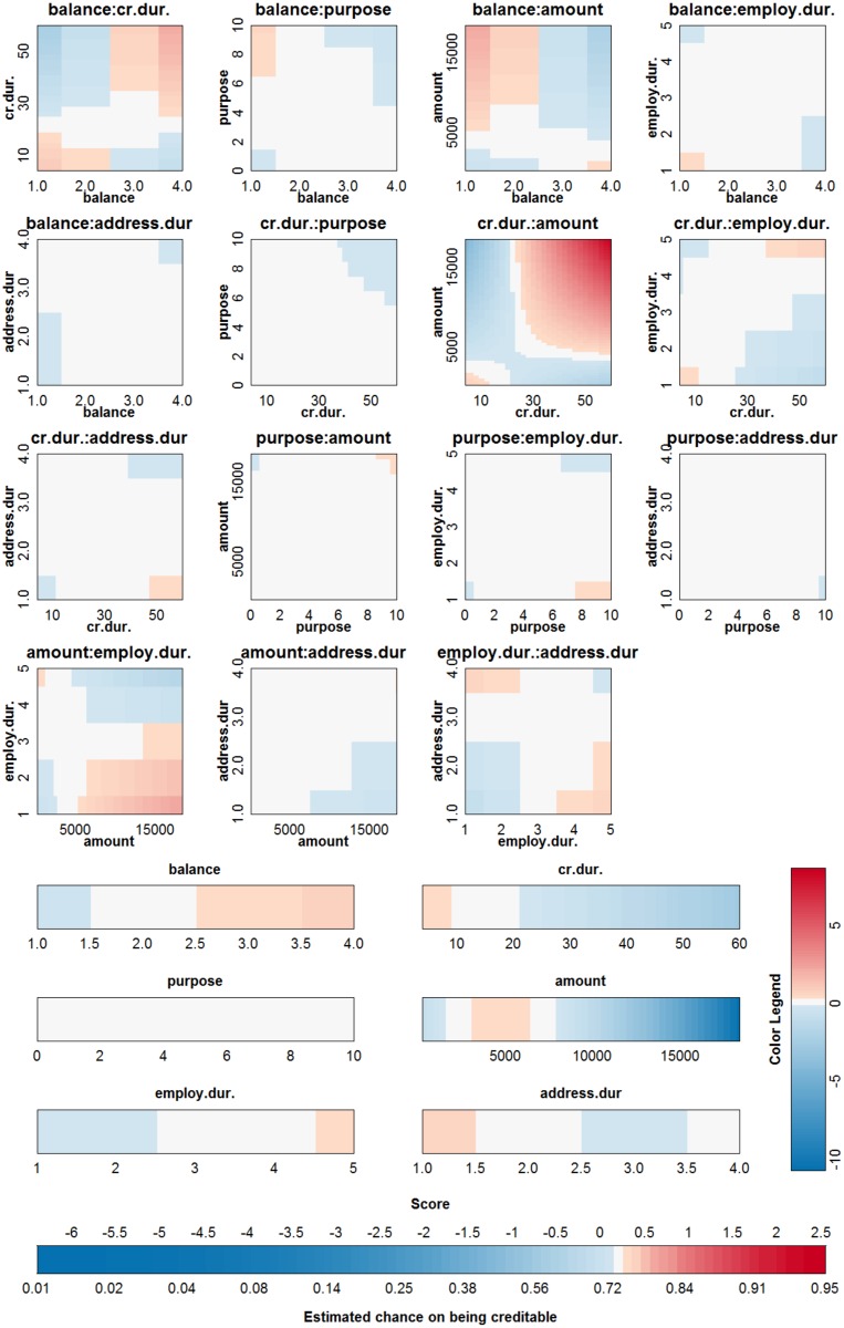
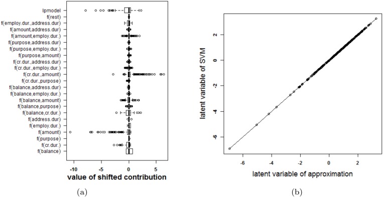
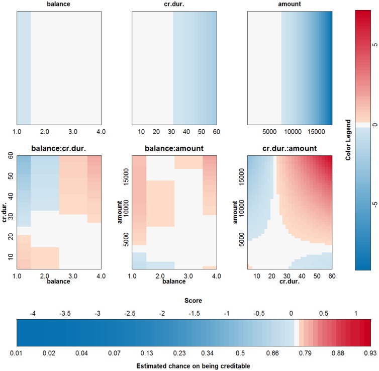
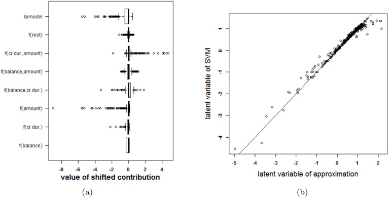
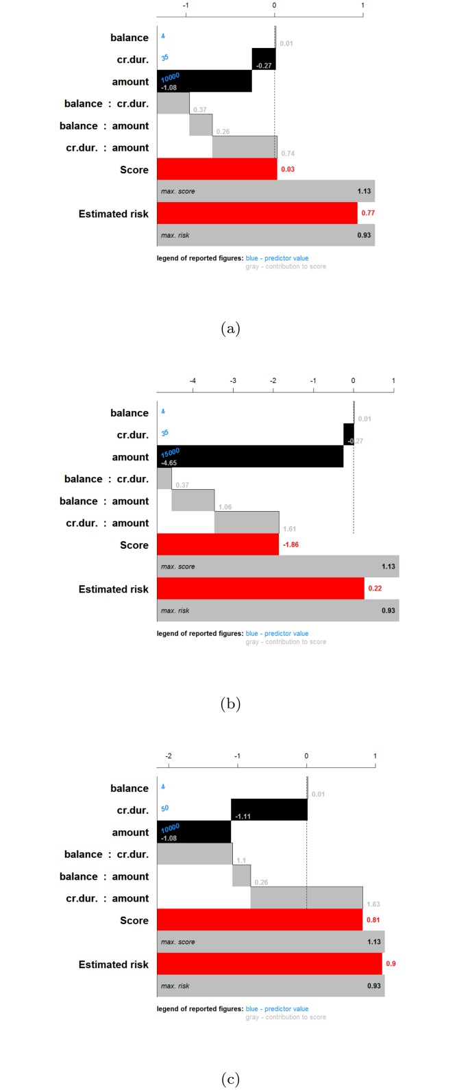
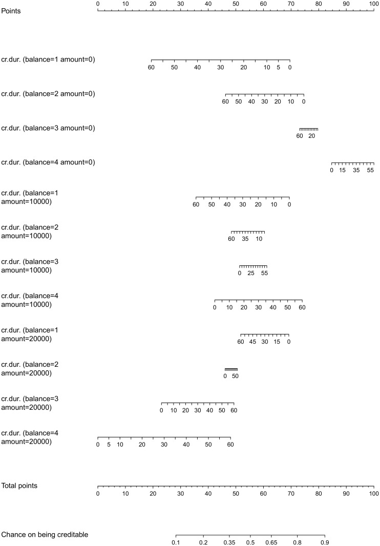
Objective: In this work, we investigate whether SVMs using linear, polynomial and RBF kernels can be explained such that interpretations for model-based decisions can be provided. We further indicate when SVMs can be explained and in which situations interpretation of SVMs is (hitherto) not possible. Here, explainability is defined as the ability to produce the final decision based on a sum of contributions which depend on one single or at most two input variables.

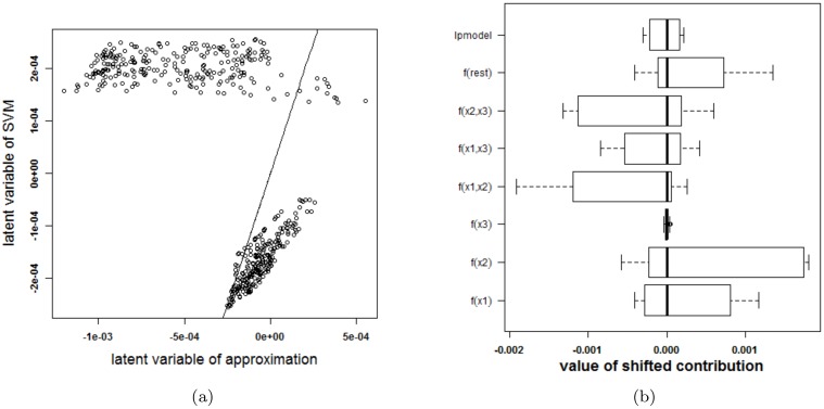
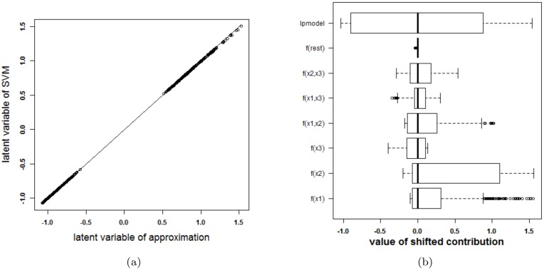
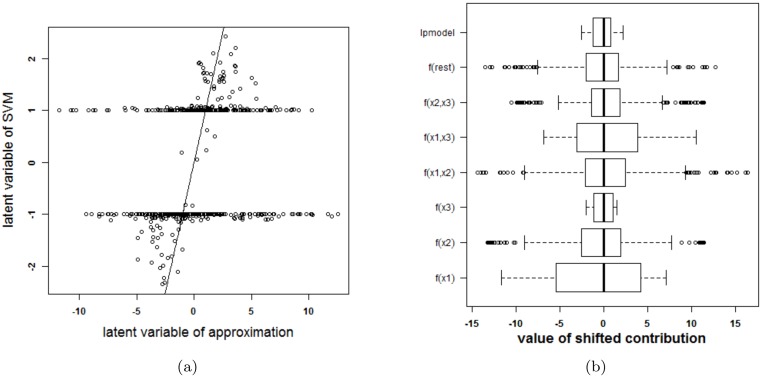
Results: Our experiments on simulated and real-life data show that explainability of an SVM depends on the chosen parameter values (degree of polynomial kernel, width of RBF kernel and regularization constant). When several combinations of parameter values yield the same cross-validation performance, combinations with a lower polynomial degree or a larger kernel width have a higher chance of being explainable.

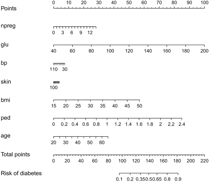
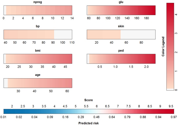
Conclusions: This work summarizes SVM classifiers obtained with linear, polynomial and RBF kernels in a single plot. Linear and polynomial kernels up to the second degree are represented exactly. For other kernels an indication of the reliability of the approximation is presented. The complete methodology is available as an R package and two apps and a movie are provided to illustrate the possibilities offered by the method.

Fig 1. Visualization of the logistic regression model for the Pima dataset by means of a nomogram.

The contribution of each input variable x^(p) (f^(p) = w^(p) x^(p)) to the linear predictor is shifted and rescaled such that each contribution has a minimal value of zero and the maximal value of all contributions is 100. Each input variable is represented by means of a scale and the value of the contribution can be found by drawing a vertical line from the input variable value to the points scale on top of the plot. Adding the contributions of all input variables results in the total points. These can be transformed into a risk estimate by drawing a vertical line from the total points scale to the risk scale. The importance of the inputs is represented by means of the length of the scales: variables with longer scales have a larger impact on the risk prediction.

Fig 2. Visualization of the logistic regression model for the Pima dataset by means of a color plot or color based nomogram.

The contribution of each input variable x^(p) (f^(p) = w^(p) x^(p)) to the linear predictor is shifted such that each contribution has a minimal value of zero. To obtain a risk estimate for an observation, the color corresponding to the input’s value needs to be indicated. This color is converted to a point by means of the color legend at the right. Repeating this for each input and summing the resulting points, yields the score. This score is then converted into the risk estimate by means of the bottom most color bar. The importance of the inputs is represented by means of the redness of the color: variables with a higher intensity in red have a larger impact on the risk prediction.

Fig 3. Performance of the approximation method (i.e. the expansion without the rest term Δℓ) on the two circles data.

(a) Latent variables of the SVM model with RBF kernel and the approximation. The approximation is not able to approximate the latent variables of the SVM model. (b) Contributions of the approximation of the SVM model and the rest term. The box-plots visualize the range of the different contributions. The upper boxplot indicates the range of the latent variable of the SVM model. In this example the range of the rest term cannot be ignored in comparison with the ranges of the other contributions. As such, the approximation of this specific SVM model cannot serve as an explanation of the SVM model.

Fig 4. Performance of the approximation method (i.e. the expansion without the rest term Δℓ) on the two circles data (second SVM model).

(a) Latent variables of the SVM model with RBF kernel and the approximation. The approximated latent variable is a good estimate of the latent variable of the SVM model. (b) Contributions of the approximation of the second SVM model and the rest term. The box-plots visualize the range of the different contributions. The upper boxplot indicates the range of the latent variable of the SVM model. In this example the range of the rest term can be ignored in comparison with the ranges of the other contributions. As such, the approximation of this specific SVM model will be able to explain the classifier.

Fig 5. Visualization of the second SVM model with RBF kernel on the example of the two circles.

Fig 6. Visualization of the third SVM model (polynomial kernel) on the example of the two circles.

Fig 7. Nomogram of a logistic regression model including polynomial transformations of the input variables for the two circles problem.

The non-linearities are visualized by the use of two axes for each input.

Fig 8. Performance of the approximation method (i.e. the expansion without the rest term Δℓ) on the swiss roll problem.

(a) Latent variables of the SVM model with RBF kernel and the approximation. The approximation is not able to approximate the latent variables of the SVM model. (b) Contributions of the approximation of the SVM model and the rest term. The box-plots visualize the range of the different contributions. The upper boxplot indicates the range of the latent variable of the SVM model. In this example the range of the rest term cannot be ignored in comparison with the ranges of the other contributions. As such, the approximation of this specific SVM model cannot serve as an explanation of the SVM model.

Fig 9. Comparison of the performance of the approximations (i.e. the expansion without the rest term Δℓ) of two SVM models on the checkerboard problem.

(a)-(c): RBF kernel, (b)-(d): polynomial kernel. (a)-(b): Latent variable of the approximation versus latent variable of the original SVM model. (c)-(d): Range of all contributions in the approximation, the rest term and the latent variable of the SVM model. For the RBF kernel, the rest term is much larger than the latent variable, resulting in an approximation that is unable to explain the SVM model. For the polynomial kernel, the rest term is negligible in comparison with the other terms and the approximation is nearly perfect.

Fig 10. Visualization of the SVM model with polynomial kernel on the checkerboard example.

It can be seen that all contributions involving x⁽³⁾ do not contribute in a large extent since the range of these contributions is very small in comparison with the other contributions.

Fig 11. Performance of the approximation method (i.e. the expansion without the rest term Δℓ) on the two Gaussians data.

(a) Latent variables of the SVM model with RBF kernel and the approximation. The approximated latent variable is a good estimate of the latent variable of the SVM model. (b) Contributions of the approximation of the SVM model and the rest term. The box-plots visualize the range of the different contributions. The upper boxplot indicates the range of the latent variable of the SVM model. In this example the range of the rest term can be ignored in comparison with the ranges of the other contributions. As such, the approximation of this specific SVM model will be able to explain the classifier.

Fig 12. Visualization of the SVM model with RBF kernel on the example of the two Gaussians.

Fig 13. Visualization of the SVM model on the IRIS data set.

Fig 14. Performance of the approximation method (i.e. the expansion without the rest term Δℓ) on the IRIS data.

(a) Boxplots of the contributions of the approximation of the SVM model, the rest term and the latent variable of the SVM model. The range of the rest term can be ignored in comparison with the ranges of the other contributions. (b) Latent variable of the original model versus those obtained from the approximation. The approximation is able to estimate the latent variable of the SVM model very accurately and as such can be used to explain the SVM model.

Fig 15. Visualization of the SVM model on the Pima data set.

Fig 16. Performance of the approximation method (i.e. the expansion without the rest term Δℓ) on the Pima data.

(a) Boxplots of the contributions of the approximation of the SVM model, the rest term and the latent variable of the SVM model. The range of the rest term can be ignored in comparison with the ranges of the other contributions. (b) Latent variable of the original model versus those obtained from the approximation. The approximation is able to estimate the latent variable of the SVM model very accurately and as such can be used to explain the SVM model.

Fig 17. Visualization of the SVM model with polynomial kernel on the German credit risk data set.

Fig 18. Performance of the approximation method (i.e. the expansion without the rest term Δℓ) on the German credit risk data.

(a) Boxplots of the contributions of the approximation of the SVM model, the rest term and the latent variable of the SVM model. The range of the rest term can be ignored in comparison with the ranges of the other contributions. (b) Latent variable of the original model versus those obtained from the approximation. The approximation is able to estimate the latent variable of the SVM model very accurately and as such can be used to explain the SVM model.

Fig 19. Visualization of the second SVM model on the German credit risk data set.

Fig 20. Performance of the approximation method (i.e. the expansion without the rest term Δℓ) on the German credit risk data (using only three inputs).

(a) Boxplots of the contributions of the approximation of the SVM model, the rest term and the latent variable of the SVM model. The range of the rest term can be ignored in comparison with the ranges of the other contributions. (b) Latent variable of the original model versus those obtained from the approximation. The approximation is able to estimate the latent variable of the SVM model accurately and as such can be used to explain the SVM model.

Fig 21. Cumulative contribution charts for three applicants to illustrate the effect of the SVM model on the German credit risk data.

The bars indicate the value of the contributions. (a) applicant 1 (balance = 4, credit duration = 35, credit amount = 10000), (b) applicant 2 (balance = 4, credit duration = 35, credit amount = 15000), (c) applicant 3 (balance = 4, credit duration = 50, credit amount = 10000).

Fig 22. Nomogram of a logistic regression model including linear main and interaction effects for the German credit risk problem with a reduced input set and 3 categories for the amount.

Interactions are dealt with by grouping main and interaction effects containing the same inputs. Interactions between continuous inputs are only possible after categorization of at least one of these inputs.

References

1. Joachims T. Learning to Classify Text Using Support Vector Machines: Methods, Theory and Algorithms; 2002. Available from: http://portal.acm.org/citation.cfm?id=572351. 10.1007/978-1-4615-0907-3 - DOI
1. Decoste D, Schölkopf B. Training invariant support vector machines. Machine Learning. 2002;46(1–3):161–190. 10.1023/A:1012454411458 - DOI
1. Moghaddam B, Yang MH. Learning gender with support faces. IEEE Transactions on Pattern Analysis and Machine Intelligence. 2002;24(5):707–711. 10.1109/34.1000244 - DOI
1. Hua S, Sun Z. Support vector machine approach for protein subcellular localization prediction. Bioinformatics (Oxford, England). 2001;17(8):721–728. 10.1093/bioinformatics/17.8.721 - DOI - PubMed
1. Van Belle V, Lisboa P. Research directions in interpretable machine learning methods. In: Verleysen M, editor. Proceedings of the European Symposium on Artificial Neural Networks, Computational Intelligence and Machine Learning (ESANN2013). d-side, Evere; 2013. p. 533–541.