Climate change and the ash dieback crisis

Abstract

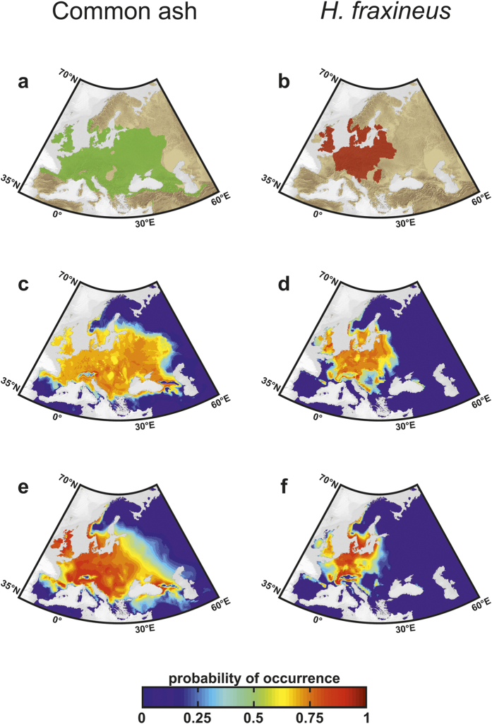
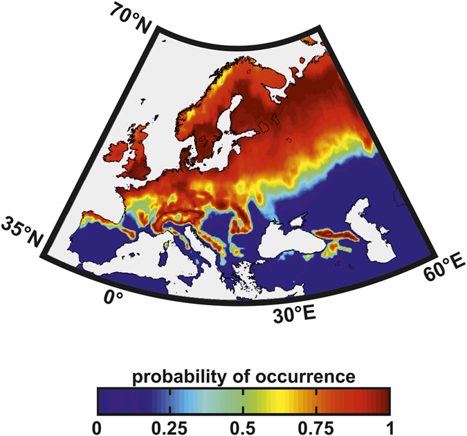
Beyond the direct influence of climate change on species distribution and phenology, indirect effects may also arise from perturbations in species interactions. Infectious diseases are strong biotic forces that can precipitate population declines and lead to biodiversity loss. It has been shown in forest ecosystems worldwide that at least 10% of trees are vulnerable to extinction and pathogens are increasingly implicated. In Europe, the emerging ash dieback disease caused by the fungus Hymenoscyphus fraxineus, commonly called Chalara fraxinea, is causing a severe mortality of common ash trees (Fraxinus excelsior); this is raising concerns for the persistence of this widespread tree, which is both a key component of forest ecosystems and economically important for timber production. Here, we show how the pathogen and climate change may interact to affect the future spatial distribution of the common ash. Using two presence-only models, seven General Circulation Models and four emission scenarios, we show that climate change, by affecting the host and the pathogen separately, may uncouple their spatial distribution to create a mismatch in species interaction and so a lowering of disease transmission. Consequently, as climate change expands the ranges of both species polewards it may alleviate the ash dieback crisis in southern and occidental regions at the same time.

Figure 1. Observed and modelled spatial distributions of common ash and its pathogen.

Observed distribution of (a) common ash (1950–2008) and (b) H. fraxineus (1992–2009) and modelled spatial distribution (as probability of occurrence) of (c,e) common ash and (d,f) H. fraxineus calculated from (c,d) MaxEnt and (e,f) NPPEN. Maps were produced using ArcGIS software v.10 (Environmental Systems Research Institute, Redlands, California, USA; http://www.esri.com/).

Figure 2. Modelled spatial distributions of Hymenoscyphus fraxineus.

Modelled spatial distribution (as probability of occurrence) of H. fraxineus calculated from a model based on the physiological tolerances of H. fraxineus to temperature using the limits defined by Hauptman et al. (see Supplementary Figure S3). Map was produced using Matlab R2015b (http://www.mathworks.com).

Figure 3. Expected long-term changes in the spatial distribution of common ash and its pathogen using MaxEnt and NPPEN.

Long-term quantitative changes (median and both first and third quartiles as shading) relative to 1992–2009 for H. fraxineus (in red), and common ash without (in green) and with (in blue) the interactive effect of H. fraxineus using (a,c,e,g) MaxEnt and (b,d,f,h) NPPEN for scenarios (a,b) RCP2.6, (c,d) RCP4.5, (e,f) RCP6.0 and (g,h) RCP8.5.

Figure 4. Expected future spatial distribution of common ash and its pathogen calculated from MaxEnt.

Projections of the averaged probability of occurrence of (a) common ash, (b) H. fraxineus and (c) common ash with consideration of the interactive effect of the pathogen (termed “common ash with H. fraxineus”) for 2080–2099 using scenarios RCP2.6, RCP4.5, RCP6.0 and RCP8.5. Maps were produced using ArcGIS software v.10 (Environmental Systems Research Institute, Redlands, California, USA; http://www.esri.com/).

Figure 5. Expected future spatial distribution of common ash and its pathogen calculated from NPPEN.

Projections of the averaged probability of occurrence of (a) common ash, (b) H. fraxineus and (c) common ash with H. fraxineus for 2080–2099 using scenarios RCP2.6, RCP4.5, RCP6.0 and RCP8.5. Maps were produced using ArcGIS software v.10 (Environmental Systems Research Institute, Redlands, California, USA; http://www.esri.com/).

References

-
- Harvell C. D. et al. Climate warming and disease risks for terrestrial and marine biota. Science 296, 2158–2162 (2002). - PubMed
- Kuussaari M. et al. Extinction debt: a challenge for biodiversity conservation. Trends Ecol Evol. 24, 564–571 (2009). - PubMed
- Altizer S., Ostfeld R. S., Johnson P. T. J., Kutz S. & Harvell C. D. Climate change and infectious diseases: From evidence to a predictive framework. Science 341, 514–519 (2013). - PubMed
- Smith M. D. An ecological perspective on extreme climatic events: a synthetic definition and framework to guide future research. J Ecol. 99, 656–663 (2011).
- Allen C. D. et al. A global overview of drought and heat-induced tree mortality reveals emerging climate change risks for forests. Forest Ecol Manag. 259, 660–684 (2010).
Publication types
MeSH terms
LinkOut - more resources
Full Text Sources
Other Literature Sources
Medical
Research Materials
Miscellaneous