Contextual Interactions in Grating Plaid Configurations Are Explained by Natural Image Statistics and Neural Modeling

Abstract

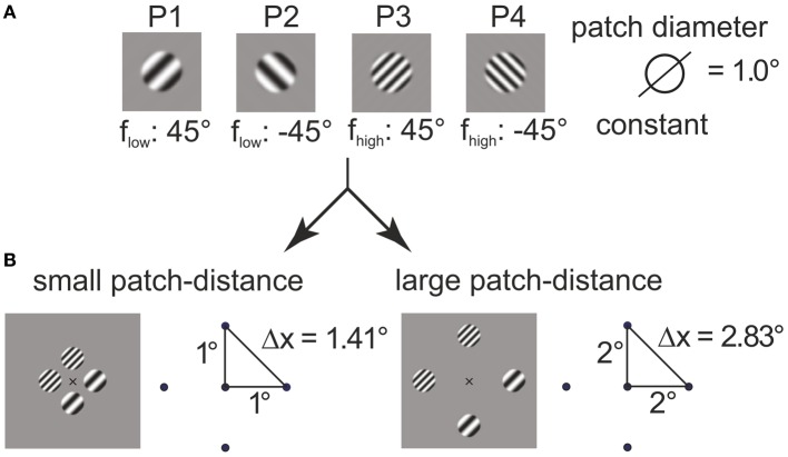
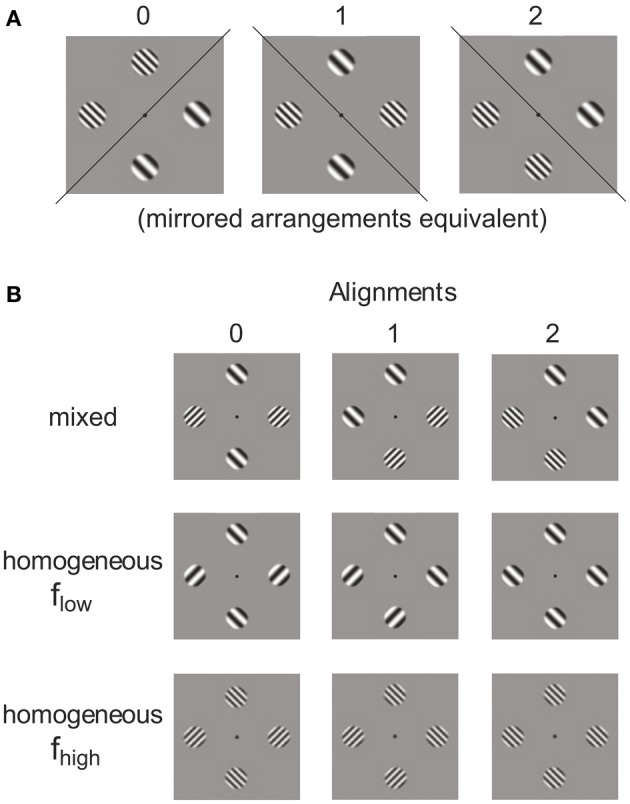
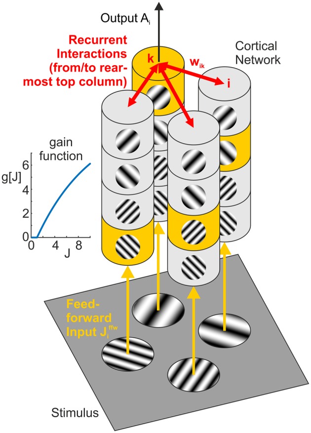
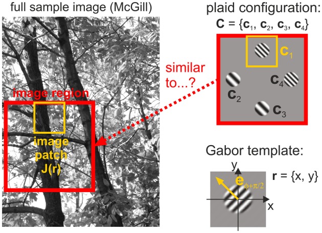
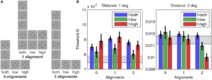
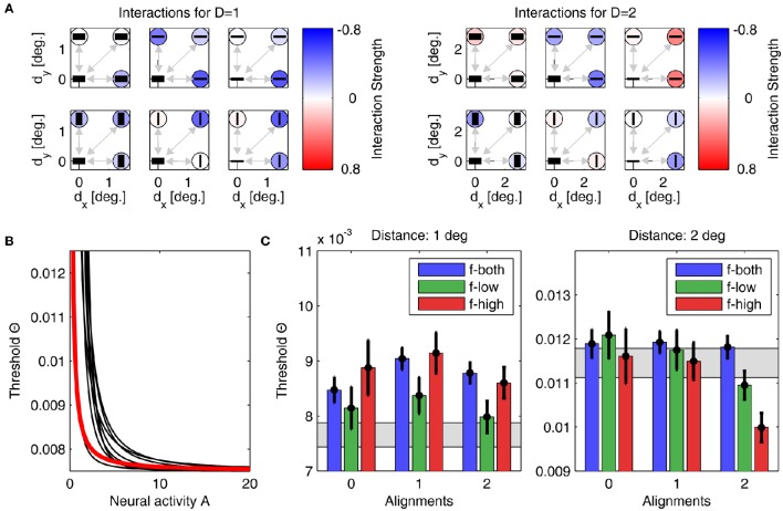
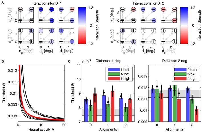
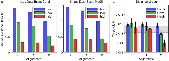
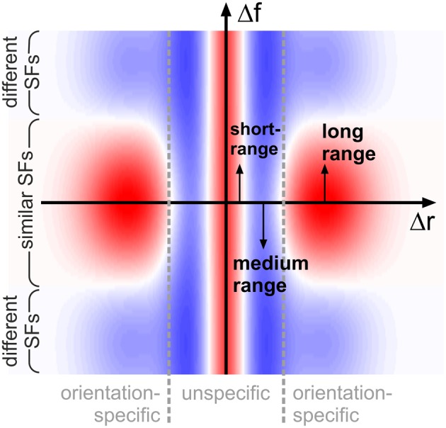
Processing natural scenes requires the visual system to integrate local features into global object descriptions. To achieve coherent representations, the human brain uses statistical dependencies to guide weighting of local feature conjunctions. Pairwise interactions among feature detectors in early visual areas may form the early substrate of these local feature bindings. To investigate local interaction structures in visual cortex, we combined psychophysical experiments with computational modeling and natural scene analysis. We first measured contrast thresholds for 2 × 2 grating patch arrangements (plaids), which differed in spatial frequency composition (low, high, or mixed), number of grating patch co-alignments (0, 1, or 2), and inter-patch distances (1° and 2° of visual angle). Contrast thresholds for the different configurations were compared to the prediction of probability summation (PS) among detector families tuned to the four retinal positions. For 1° distance the thresholds for all configurations were larger than predicted by PS, indicating inhibitory interactions. For 2° distance, thresholds were significantly lower compared to PS when the plaids were homogeneous in spatial frequency and orientation, but not when spatial frequencies were mixed or there was at least one misalignment. Next, we constructed a neural population model with horizontal laminar structure, which reproduced the detection thresholds after adaptation of connection weights. Consistent with prior work, contextual interactions were medium-range inhibition and long-range, orientation-specific excitation. However, inclusion of orientation-specific, inhibitory interactions between populations with different spatial frequency preferences were crucial for explaining detection thresholds. Finally, for all plaid configurations we computed their likelihood of occurrence in natural images. The likelihoods turned out to be inversely related to the detection thresholds obtained at larger inter-patch distances. However, likelihoods were almost independent of inter-patch distance, implying that natural image statistics could not explain the crowding-like results at short distances. This failure of natural image statistics to resolve the patch distance modulation of plaid visibility remains a challenge to the approach.

Keywords: contextual interactions; feature integration; natural image statistics; network model; visual cortex; visual perception.

Figure 1

Construction of plaids from grating patches. The four grating patches (A) used for 4–plaid configurations in small and large inter-patch distance (B).

Figure 2

Categories of plaids. Different grating patch configurations obtained from allocating two pairs of patches to four locations (A) and alignment variation in frequency–homogeneous and inhomogeneous patch compositions (B).

Figure 3

Network model. Feedforward input from the visual stimulus (bottom) activates neural columns (marked in yellow) with matching orientation and spatial frequency (SF) preference in each of the four hypercolumns (vertical structures). Horizontal interactions (in red) provide recurrent feedback between different (hyper-)columns in the network. Note that for clarity, we only show connections originating from the top column in the rearmost hypercolumn, targeting columns with the same orientation and SF preference in the neighboring three hypercolumns (i.e., the set of interactions shown in the top left subpanel of Figures 6, 7). The inset graph shows the neural gain function g[J] mapping a synaptic input J to a neural population response.

Figure 4

Image analysis. Image regions taken from a full image converted to gray scale (left) are compared with plaid configurations (top right) by comparing Gabor templates (bottom right) with different spatial frequencies and different orientations to image patches (yellow outlines) positioned at the four positions in a plaid.

Figure 5

Human detection thresholds for different plaid configurations. (A) The 22 plaid configurations used in the experiment, sorted according to grating patch alignment (zero alignments, one alignment, or two alignments) and SF content (only low SFs, only high SFs, or both SFs), giving nine categories in total. (B) The graph on the left shows results for plaid distance d = 1°, and the graph on the right for plaid distances of d = 2°. The height of the bars indicates the average detection threshold and the vertical black lines the corresponding 95% confidence interval. For comparison, the gray bars display the approximate detection thresholds predicted from single element detection by assuming independency and probability summation. Bars significantly above the gray region thus indicate suppressive interactions, while bars significantly below indicate facilitating interactions.

Figure 6

Parameters and performance of model A. For this figure, we used the parameter set yielding model results best matching the experimental data. (A) Interactions for plaid distances d = 1° (left) and d = 2° (right). The six subplots corresponding to each plaid distance show interactions between the neuronal unit in the lower left corner to all other units, with their orientation preferences and SFs indicated by the black bars (thick bar for low SF, thin bar for high SF). Interaction strength is color coded (insides of circles). The upper row displays all interactions for units with similar orientation preferences, while the lower row displays interactions between units with orthogonal orientation preferences. The outer columns display interactions between units with similar SFs, while the middle column displays interactions between units with different SFs. For simplifying the figure, the original plaid configuration has been rotated by 45 degrees. (B) Mapping of activities onto thresholds for the 'best' model (thick red line), and for nine other models with the next-best performances (thin black lines). (C) Comparison of detection thresholds from model and experiment for plaid distances d = 1° (left) and d = 2° (right). The predicted thresholds from the model are displayed as colored bars (color code as inset), while the psychophysical thresholds are indicated by the black circles with the vertical lines showing the corresponding 95%-confidence intervals. The region shaded in gray color indicates the range of thresholds expected from probability summation. Note that model predictions and actual thresholds are indistinguishable from each other.

Figure 7

Parameters and performance of model B. We again use the parameter set yielding the best matching results. Display as in Figure 6. Although match of model to experiment is not as good as before, still only one model prediction is outside the confidence interval.

Figure 8

Results of image analysis compared to human psychophysics. (A) The height of the bars indicates the inverse of the average likelihood ratio Λ for the corresponding plaid configurations, sorted into the same categories as used in Figure 5 for showing the psychophysics results. The left graph and right graphs show the results for the Corel and McGill data bases, respectively. For comparison, (B) shows the experimental results for d = 2° (same as in Figure 5, right graph), which come closest to the observed result pattern.

Figure 9

Schematic representation of interactions. Coupling scheme implied by our findings, shown for feature detectors with similar orientation preferences: antagonistic interactions in space (on small and intermediate distances Δr, horizontal axis) are complemented by antagonistic interactions in spatial frequency (vertical axis, Δf) for long spatial distances. Excitatory and inhibitory interactions are shown in red and blue shading, respectively. For clarity of illustration, we do not show that interaction length scales in addition depend on spatial frequency.

References

1. Adini Y., Sagi D., Tsodyks M. (1997). Excitatory-inhibitory network in the visual cortex: psychophysical evidence. Proc. Natl. Acad. Sci. U.S.A. 94, 10426–10431. 10.1073/pnas.94.19.10426 - DOI - PMC - PubMed
1. Bex P. J., Simmers A. J., Dakin S. C. (2001). Snakes and ladders: the role of temporal modulation in visual contour integration. Vis. Res. 41, 3775–3782. 10.1016/S0042-6989(01)00222-X - DOI - PubMed
1. Bosking W. H., Zhang Y., Schofield B., Fitzpatrick D. (1997). Orientation selectivity and the arrangement of horizontal connections in tree shrew striate cortex. J. Neurosci. 17, 2112–2127. - PMC - PubMed
1. Bruchmann M., Breitmeyer B. G., Pantev C. (2010). Metacontrast masking within and between visual channels: effects of orientation and spatial frequency contrasts. J. Vis. 10, 1–14. 10.1167/10.6.12 - DOI - PubMed
1. Callaway E. M. (2004). Feedforward, feedback and inhibitory connections in primate visual cortex. Neural Netw. 17, 625–632. 10.1016/j.neunet.2004.04.004 - DOI - PubMed
LinkOut - more resources