. 2016 Aug 30;3(4):ENEURO.0085-16.2016.
doi: 10.1523/ENEURO.0085-16.2016. eCollection 2016 Jul-Aug.

The Largest Response Component in the Motor Cortex Reflects Movement Timing but Not Movement Type

Affiliations

The Largest Response Component in the Motor Cortex Reflects Movement Timing but Not Movement Type

Matthew T Kaufman et al. eNeuro. .

Abstract

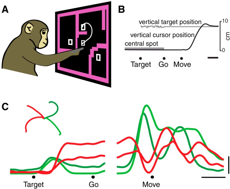
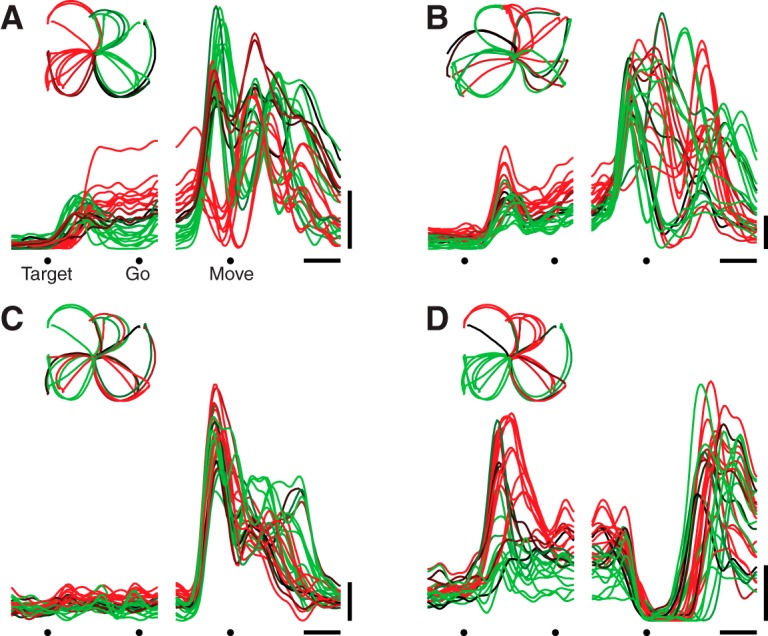
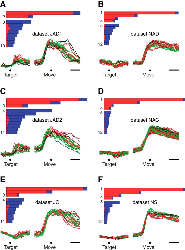
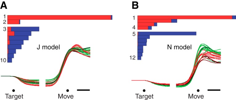
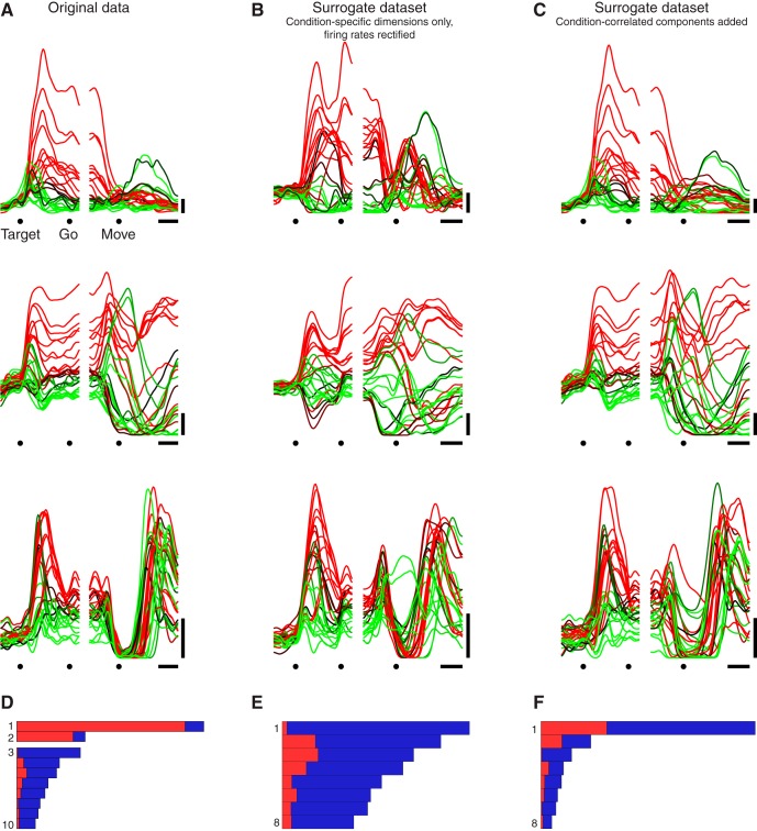
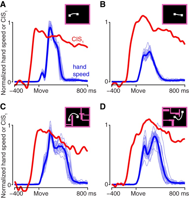
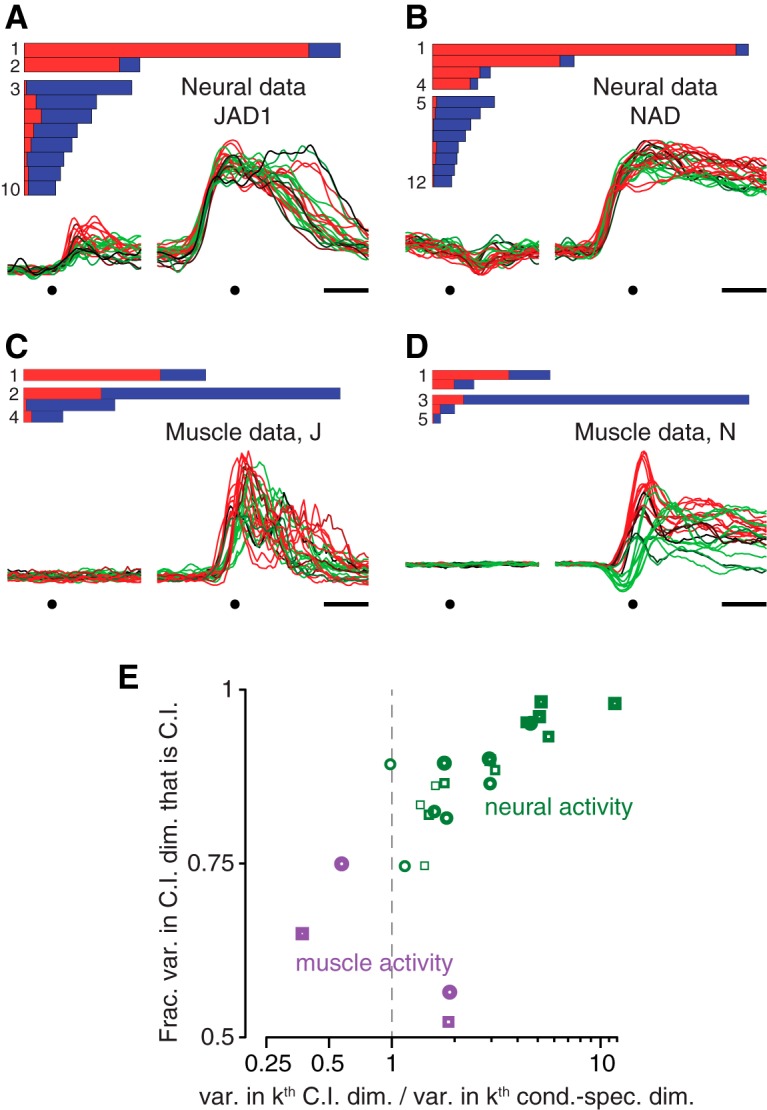
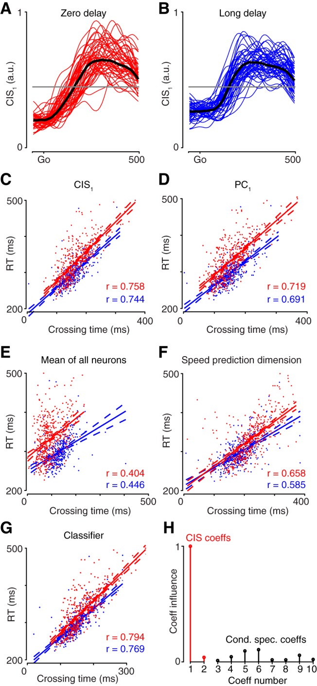
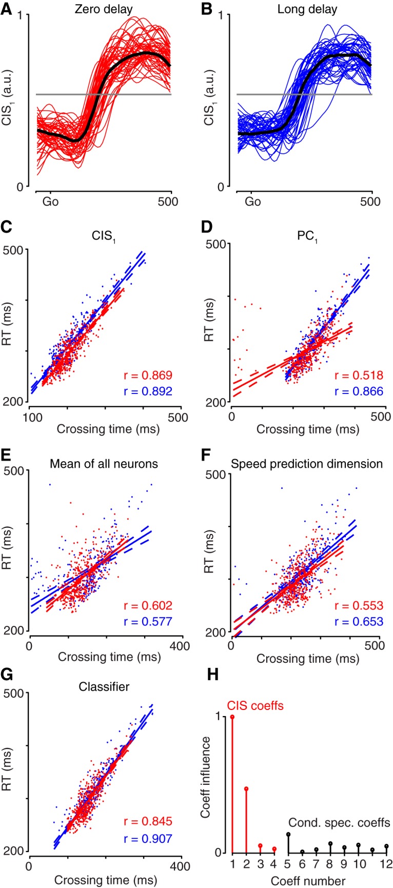
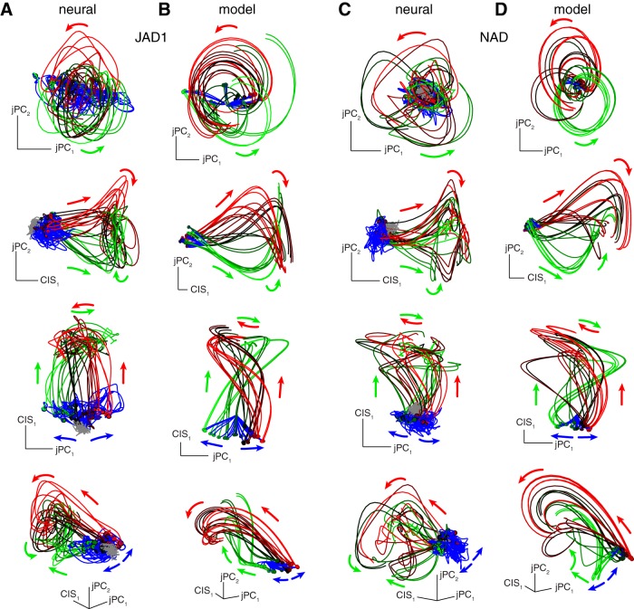
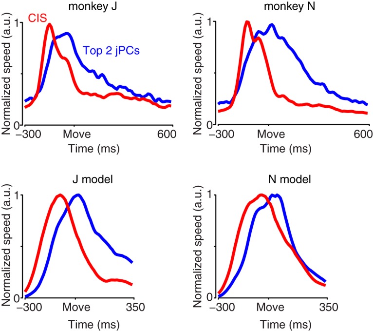
Neural activity in monkey motor cortex (M1) and dorsal premotor cortex (PMd) can reflect a chosen movement well before that movement begins. The pattern of neural activity then changes profoundly just before movement onset. We considered the prediction, derived from formal considerations, that the transition from preparation to movement might be accompanied by a large overall change in the neural state that reflects when movement is made rather than which movement is made. Specifically, we examined "components" of the population response: time-varying patterns of activity from which each neuron's response is approximately composed. Amid the response complexity of individual M1 and PMd neurons, we identified robust response components that were "condition-invariant": their magnitude and time course were nearly identical regardless of reach direction or path. These condition-invariant response components occupied dimensions orthogonal to those occupied by the "tuned" response components. The largest condition-invariant component was much larger than any of the tuned components; i.e., it explained more of the structure in individual-neuron responses. This condition-invariant response component underwent a rapid change before movement onset. The timing of that change predicted most of the trial-by-trial variance in reaction time. Thus, although individual M1 and PMd neurons essentially always reflected which movement was made, the largest component of the population response reflected movement timing rather than movement type.

Keywords: condition-invariant signal; dPCA; movement initiation; movement triggering; reaction time; state space.


Conflict of interest statement

The authors report no conflict of interest.

Figures

Figure 1.
Figure 1.
Task and basic neural responses. A, B, Illustration of the maze task. Monkeys executed reaches that avoided any intervening barriers. The task was performed with a cursor presented just above the monkey’s hand. White trace shows the path of the cursor on one trial. Target, Target onset; Go, go cue; Move, movement onset. C, PSTH for an example neuron for four (of 27) conditions. Each trace shows the trial-averaged firing rate for one reach condition (one unique maze) over time. Averaging was performed twice: locked to target onset (left traces) and movement onset (right traces). Only trials with a 500 ms delay were included. Inset, Reach trajectories, colored the same as their corresponding neural traces. This neuron illustrates the transition between stable preparatory activity and rapidly changing movement-related activity. Scale bars: B, C, horizontal, 200 ms; C, vertical, 10 spikes/s.
Figure 2.
Figure 2.
Responses of four example neurons. Format is as in Figure 1C, but responses are shown for all 27 conditions. A, Unit with complex responses. This neuron showed both an overall increase in firing rate across conditions and a strong oscillatory component that was condition-specific (unit JAD1-98, same as in Fig. 1C). Scale bars same as Figure 1C. Inset in upper left shows reach trajectories, colored the same as their corresponding neural traces. B, Another unit with complex condition-specific responses, recorded from the other monkey (unit NAD-165). C, Unit with responses that were strongly condition-correlated (unit JAD1-70). D, Unit where the initial response was condition-correlated: a decline across all conditions. Later activity is more condition-specific (unit JAD1-114).
Figure 3.
Figure 3.
Performance of demixing on the empirical data. A. Bars show the relative variance captured by each dPCA component for dataset JAD1. Each bar’s horizontal extent indicates the total variance captured by that component. The red portion indicates condition-invariant variance, while the blue portion indicates condition-specific variance. Components are grouped according to whether they were overall condition-invariant (top group, >50% condition-invariant variance) or condition-specific (bottom group, >50% condition-specific variance). Traces show the projection onto the first dimension found by dPCA (CIS1) versus time. Each trace corresponds to one condition. Target, target onset; Move, movement onset. Scale bars, 200 ms. B—F. Same as A, for the remaining datasets.
Figure 4.
Figure 4.
Same as Figure 3, but for the recurrent neural network models.
Figure 5.
Figure 5.
Demixing performance for one empirical dataset and two surrogate control datasets. A, PSTHs of three example units from dataset JAD1. Scale bars: horizontal, 200 ms; vertical, 10 spikes/s. B, PSTHs for a surrogate dataset where we projected onto the condition-specific dimensions, then rectified so that all firing rates remained positive (see Materials and Methods). This surrogate dataset explores the possibility that a CIS might appear merely due to firing rates being constrained to be positive. The three PSTHs correspond to the same units shown in A, after modification. C, PSTHs for a surrogate dataset where we added condition-correlated components. The condition-correlated components had the same temporal profile as the projections onto the condition-invariant dimensions found by dPCA but had a different amplitude for each condition (see Materials and Methods). This surrogate dataset explores whether a condition-correlated structure at the single-neuron level is sufficient to yield condition-invariant components at the population level. The three PSTHs correspond to the same units shown in A, after modification. D–F. Quantification of the CIS as in Figure 3. Panels correspond to examples above. D is reproduced from Figure 3A for comparison.
Figure 6.
Figure 6.
Comparison of the CIS and hand speed. Hand speed (blue) and the first component of the CIS (red) are shown for four reach conditions. For hand speed, light traces show all trials; heavy trace shows mean over trials. CIS1 is the mean over trials. Insets show the maze for that condition and a prototypical reach path. A, A straight reach with a fast speed profile. Maze ID25. B, A straight reach with a slow speed profile. Maze ID7. C, A curved reach with a long speed profile. Maze ID5. D, A curved reach with an unusual speed profile. Maze ID14. The CIS was similar across all four examples, despite differences in the speed profile. Dataset NAD.
Figure 7.
Figure 7.
Comparison of dPCA applied to neural and muscle populations. A, B, Demixing performance (bars) and the projection onto the first dimension found by dPCA (CIS1) for neural datasets JAD1 and NAD. Each trace corresponds to one condition. These panels are reproduced from Figure 3A,B for comparison with the corresponding analysis of EMG. Dots indicate target onset and movement onset. Scale bar, 200 ms. C, D, Similar analysis as in A and B, but for the muscle populations recorded for monkeys J and N. Muscle activity was recorded for the same sets of conditions as for the neural data in A and B. E, To compare the prevalence of a condition-invariant structure in the neural and muscle populations, we focused on nominally “condition-invariant” components with >50% condition-invariant variance. There were many such components for the neural populations (green) and 1–2 such components for each of the muscle populations (purple). For each such component, two measurements were taken: the fraction of the component’s variance that was condition-invariant (vertical axis) and the total variance captured. The latter was expressed in normalized terms: the variance captured by the k th nominally “condition-invariant” component divided by the total variance captured by the k th “condition-specific” component (horizontal axis). Only the neural datasets contained components that were both strongly condition-invariant (high on the vertical axis) and that captured relatively large amounts of variance (to the right on the horizontal axis). Heaviest symbols correspond to the first dimension found by dPCA for each dataset; higher-numbered dimensions are plotted as progressively lighter symbols. Dashed gray line highlights variance ratio of unity. Circles, monkey J datasets; squares, monkey N datasets.
Figure 8.
Figure 8.
Predicting RT using projections of the data for dataset JAD1. A, Each trace plots CIS1 over time on a single zero-delay trial. Fifty trials selected randomly at intervals throughout the day are shown. Black trace plots the median across all trials. B, Same as in A but for trials with a 500 ms delay period (long delay). The criterion value (gray line) was chosen using long-delay trials. The same value was used for zero-delay trials (A). C–G, Correlation of behavioral RT with the time when the neural criterion value was crossed. For each panel, data are shown for both long-delay trials (blue) and zero-delay trials (red). Lines show linear regressions; dashed lines show 95% confidence bounds of the fit. Each panel in C–G gives the correlation for a different linear projection of the population response: CIS1 (C), the projection onto the first PC (D), the mean over all neurons (E), the projection onto the dimension that best reconstructed speed according to a linear regression (F), and the projection onto the axis found by a logistic regression classifier (G). Trials where the neural data did not cross the criterion value were excluded. H, Coefficient influence for the classifier. Coefficients for condition-invariant dimensions shown in red; condition-specific dimensions shown in black.
Figure 9.
Figure 9.
Predicting RT using projections of the data for dataset NAD. Same format as Figure 8. Regarding H, note that for this dataset there were four CIS components.
Figure 10.
Figure 10.
Various projections that capture CIS1 and rotations of the neural state during movement. Data were first projected onto three dimensions: the dimension that yielded CIS1 and two condition-specific dimensions that captured strong rotational structure (see Materials and Methods). Each panel plots a different view of the data projected onto those three dimensions. A, Four different views of the three-dimensional projection for dataset JAD1. “Baseline” activity (before target onset) plotted in gray, preparatory activity plotted in blue, and activity after the go cue plotted in green and red (colors chosen arbitrarily for each condition). B, Same for the neural network model trained to produce EMG recorded from monkey J. C, Same for dataset NAD. D, Same for the neural network model trained to produce EMG recorded from monkey N.
Figure 11.
Figure 11.
Comparison of the temporal profile of the trajectory of the CIS and the temporal profile of the condition-specific rotational patterns. The vertical axis plots “neural speed”: the rate of change of the neural state in the condition-invariant dimensions (red) and in the first jPCA plane (blue), which captures the strongest rotations. The rate of change was computed separately for each condition, then averaged across conditions. For each dataset that average was normalized by its maximum. For statistical power, results for the neural data were averaged across the three datasets for each monkey. Move, Movement onset. Note that because the data have been smoothed and differentiated, the first moment when the state begins to change is shifted leftwards: the CIS appears to begin changing >200 ms before movement onset, when ∼150 ms is a more accurate estimate (Fig. 3). Since both the condition-invariant dimensions and the jPCA dimensions are processed in the same way, however, their relative timing can be compared.

Similar articles

Cited by

References

    1. Ames KC, Ryu SI, Shenoy KV (2014) Neural dynamics of reaching following incorrect or absent motor preparation. Neuron 81:438–451. 10.1016/j.neuron.2013.11.003 - DOI - PMC - PubMed
    1. Bastian A, Schöner G, Riehle A (2003) Preshaping and continuous evolution of motor cortical representations during movement preparation. Eur J Neurosci 18:2047–2058. - PubMed
    1. Brendel W, Romo R, Machens C (2011) Demixed principal component analysis. Adv Neural Info Process Syst 24:1–9.
    1. Chase SM, Schwartz AB (2011) Inference from populations: going beyond models. Prog Brain Res 192:103–112. 10.1016/B978-0-444-53355-5.00007-5 - DOI - PubMed
    1. Churchland AK, Kiani R, Shadlen MN (2008) Decision-making with multiple alternatives. Nat Neurosci 11:693–702. 10.1038/nn.2123 - DOI - PMC - PubMed

Publication types