Effects of quasiperiodic forcing in epidemic models

Abstract

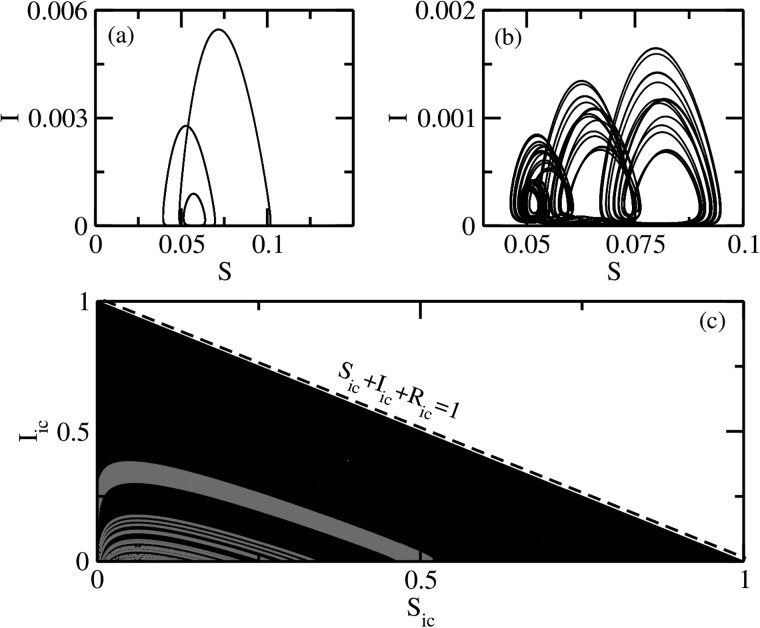
We study changes in the bifurcations of seasonally driven compartmental epidemic models, where the transmission rate is modulated temporally. In the presence of periodic modulation of the transmission rate, the dynamics varies from periodic to chaotic. The route to chaos is typically through period doubling bifurcation. There are coexisting attractors for some sets of parameters. However in the presence of quasiperiodic modulation, tori are created in place of periodic orbits and chaos appears via finite torus doublings. Strange nonchaotic attractors (SNAs) are created at the boundary of chaotic and torus dynamics. Multistability is found to be reduced as a function of quasiperiodic modulation strength. It is argued that occurrence of SNAs gives an opportunity of asymptotic predictability of epidemic growth even when the underlying dynamics is strange.

FIG. 1.

Time-dependent reproductive ratio $R_0(t)=\frac{\beta (t)}{(\mu +\eta )}$ as a function of time (see Eq. (4)) for two different δ and $ϵ$ combinations: (a) $\delta =0.2471,ϵ=0.01$ and (b) $\delta =0.184,ϵ=1$.

FIG. 2.

The δ–$ϵ$ parameter space for the quasiperiodically forced SIR model. The red regions are of chaotic (C) dynamics while white indicates periodic or regular torus (T) dynamics. The strange nonchaotic attractors lie at the regular–chaos boundary (green). These regions were demarcated using the largest nonzero Lyapunov exponent.

FIG. 3.

The coexistence of multiple attractors in terms of long-term dynamics of the periodically forced SIR model. Bifurcation diagrams are shown as a function of modulation parameter δ in Eq. (4) with $ϵ=0.0$ in the forward (a) and backward (b) directions. The corresponding two nonzero largest Lyapunov exponents (red and green) are shown in (c) and (d). The coexistence or multistability of attractors can be observed from the bifurcation diagrams as well as the Lyapunov exponents.

FIG. 4.

Coexisting periodic and chaotic attractors for the periodically forced SIR model and their basins: (a) periodic attractor, (b) chaotic attractor, and (c) the basins belonging to two distinct attractors–the red regions are the basin of attraction for the attractor in (a) while the black regions the basin of attraction of the attractor in (b). Here, the parameters are fixed at $\delta =0.25$ with $ϵ$ = 0 (only periodic modulation), $\mu =0.02$, and η = 100.

FIG. 5.

Long-term dynamics of the quasiperiodically forced SIR model. Bifurcation diagrams are shown as a function of δ in Eq. (4) with $ϵ=0.01$ (a) and $ϵ$ = 1 (b). The corresponding largest nonzero Lyapunov exponents are shown in (c) and (d). The data shown in black and red, respectively, were obtained by the forward and backward procedures. The boxes formed by the difference in the forward and backward Lyapunov exponent indicate multistability, some of which can be seen from the bifurcation diagrams as well. Clearly there are no indication of multistability at $ϵ$ = 1. The little arrows in (c) and (d) indicate the parameter values around which SNAs are found (see Figs. 6 and 8).

FIG. 6.

Three types of dynamics in the quasiperiodic SIR model. The trajectory types for $ϵ$ = 1 and different δ values are as follows: (a) a regular torus at $\delta =0.165$, (b) an SNA at $\delta =0.18$, and (c) a chaotic orbit at $\delta =0.184$. The plots (d)–(f) show the respective phase sensitivity parameter, over different initial conditions, as a function of trajectory length showing that the trajectory in (a) is smooth while those shown in (b) and (c) are non-smooth. The plots (g)–(i) show the distribution of finite time largest Lyapunov exponents, $P({\lambda }_1,t)$ with t = 1000. The sensitivity exponent defined in Eq. (6) is q = 0 for the torus in (a) and $q\sim 1.82$ for SNA in (b) as obtained by curve fitting. The chaotic orbit shows a growth of the form $\Gamma (t)\sim e^{\mathit{q}\mathit{t}}$ with $q\sim 2.43$. The curve for $\Gamma (t)$ along with best fits is shown in black.

FIG. 7.

(a) The largest nonzero Lyapunov exponent and (b) the mean square displacement $⟨r^2⟩$ as a function of $ϵ$ at $\delta =0.277$ obtained for the dynamics of the quasiperiodically forced SIR model. Note that both diagrams indicate that multistability disappears after a critical $ϵ$_c marked by black arrows.

FIG. 8.

(a) SNA observed at $\delta =0.2471,ϵ=0.01$ in the quasiperiodically forced SIR model. (b) Its phase sensitivity parameter over different initial conditions, and (c) basin of attraction, indicating that no other orbits coexist with it at this point in the parameter space. The other parameters are fixed at $\mu =0.02,\eta =100$.

FIG. 9.

The δ–$ϵ$ parameter space for the quasiperiodically forced SIRS model. The red regions are of chaotic dynamics while the white region indicates torus or periodic dynamics. The strange nonchaotic attractors lie at the regular–chaos boundary (not shown). These regions were demarcated using the largest nonzero Lyapunov exponent. The chaotic regions decrease as κ is changed from (a) 0.001, (b) 0.01, (c) 0.02, and (d) 0.03.

FIG. 10.

The δ–$ϵ$ parameter space for the quasiperiodically forced SEIR model. The red regions are of chaotic dynamics while the white region indicates torus or periodic dynamics. The strange nonchaotic attractors lie at the regular–chaos boundary (not shown). These regions were demarcated using the largest nonzero Lyapunov exponent. The parameter σ varies from (a) 35.8423, (b) 15.0, and (c) 8.0. The chaotic regions gradually become narrower as σ is decreased.

References

1. Altizer S., Dobson A., Hosseini P., Hudson P., Pascual M., and Rohani P., Ecol. Lett. 9, 467 (2006).10.1111/j.1461-0248.2005.00879.x - DOI - PubMed
1. Grassly N. C. and Fraser C., Proc. R. Soc. London, B 273, 2541 (2006).10.1098/rspb.2006.3604 - DOI - PMC - PubMed
1. Fisman D. N., Annu. Rev. Public Health 28, 127 (2007).10.1146/annurev.publhealth.28.021406.144128 - DOI - PubMed
1. Anderson R. M. and May R. M., Infectious Diseases of Humans: Dynamics and Control ( Oxford University Press, Oxford, 1992).
1. Keeling M. J. and Rohani P., Modelling Infectious Diseases in Humans and Animals ( Princeton University Press, Princeton, 2008).
LinkOut - more resources