Tensor Analysis Reveals Distinct Population Structure that Parallels the Different Computational Roles of Areas M1 and V1

Abstract

Cortical firing rates frequently display elaborate and heterogeneous temporal structure. One often wishes to compute quantitative summaries of such structure-a basic example is the frequency spectrum-and compare with model-based predictions. The advent of large-scale population recordings affords the opportunity to do so in new ways, with the hope of distinguishing between potential explanations for why responses vary with time. We introduce a method that assesses a basic but previously unexplored form of population-level structure: when data contain responses across multiple neurons, conditions, and times, they are naturally expressed as a third-order tensor. We examined tensor structure for multiple datasets from primary visual cortex (V1) and primary motor cortex (M1). All V1 datasets were 'simplest' (there were relatively few degrees of freedom) along the neuron mode, while all M1 datasets were simplest along the condition mode. These differences could not be inferred from surface-level response features. Formal considerations suggest why tensor structure might differ across modes. For idealized linear models, structure is simplest across the neuron mode when responses reflect external variables, and simplest across the condition mode when responses reflect population dynamics. This same pattern was present for existing models that seek to explain motor cortex responses. Critically, only dynamical models displayed tensor structure that agreed with the empirical M1 data. These results illustrate that tensor structure is a basic feature of the data. For M1 the tensor structure was compatible with only a subset of existing models.

Fig 1. Illustration of the stimuli/task and neural responses for one V1 dataset and one M1 dataset.

(a) Responses of four example neurons for a V1 dataset recorded via an implanted electrode array during presentation of movies of natural scenes. Each colored trace plots the trial-averaged firing rate for one condition (one of 25 movies). For visualization, traces are colored red to blue based on the firing rate early in the stimulus. (b) Responses of four example neurons for an M1 dataset recorded via two implanted electrode arrays during a delayed-reach task (monkey J). Example neurons were chosen to illustrate the variety of observed responses. Each colored trace plots the trial-averaged firing rate for one condition; i.e., one of 72 straight and curved reach trajectories. For visualization, traces are colored based on the firing rate during the delay period between target onset and the go cue. Insets show the reach trajectories (which are the same for each neuron) using the color-coding for that neuron. M1 responses were time-locked separately to the three key events: target onset, the go cue, and reach onset. For presentation, the resulting average traces were spliced together to create a continuous firing rate as a function of time. However, the analysis window included primarily movement-related activity. Gray boxes indicate the analysis windows (for V1, T = 91 time points spanning 910 ms; for M1, T = 71 time points spanning 710 ms). Horizontal bars: 200 ms; vertical bars: 20 spikes per second.

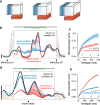
Fig 2. Schematic illustration of population tensor and results of a simplified preferred-mode analysis for two datasets.

(a) The population response can be represented as firing rate values arranged in an N × C × T array, i.e. a third-order tensor indexed by neuron, condition, and time. That population tensor (left) can be thought of as a collection of C × T matrices (one for each neuron, middle) or a collection of N × T matrices (one for each condition, right). (b) The population tensor may be approximately reconstructed (via linear combinations) from a set of ‘basis-neurons’ (C × T matrices, red) or from a set of ‘basis-conditions’ (N × T matrices, blue). Depending on the nature of the data, the basis-neurons or the basis-conditions may provide the better reconstruction. (c) Normalized reconstruction error of the population tensors for the V1 and M1 datasets shown in Fig 1when reconstructed using basis neurons (red) or basis conditions (blue). Error bars show the standard errors across conditions (Methods). The number of basis elements (12 for V1 and 25 for M1) was the same for the neuron and condition modes and was chosen algorithmically (Methods). Robustness of the preferred mode with respect to the number of basis elements is shown in subsequent analyses.

Fig 3. Illustration of the full preferred-mode analysis.

Reconstruction error is measured as a function of the number of times included in the population tensor. (a) Schematic of the method. A fixed number (three in this simple illustration) of basis-neurons (red) and basis-conditions (blue) is used to reconstruct the population tensor. This operation is repeated for different subsets of time (i.e., different sizes of the population tensor) three of which are illustrated. Longer green brackets indicate longer timespans. (b) The firing rate (black) of one example V1 neuron for one condition, and its reconstruction using basis-neurons (red) and basis-conditions (blue). Short red/blue traces show reconstructions when the population tensor included short timespans. Longer red/blue traces show reconstructions when the population tensor was expanded to include longer timespans. Dark red/blue traces show reconstructions when the population tensor included all times. For illustration, data are shown for one example neuron and condition, after the analysis was applied to a population tensor that included all neurons and conditions (same V1 dataset as in Figs 1A and 2C). The dashed box indicates the longest analyzed timespan. Responses of the example neuron for other conditions are shown in the background for context. Vertical bars: 10 spikes per second. (c) Plot of normalized reconstruction error (averaged across all neurons and conditions) for the V1 dataset analyzed in b. Red and blue traces respectively show reconstruction error when using 12 basis neurons and 12 basis conditions. The horizontal axis corresponds to the duration of the timespan being analyzed. Green arrows indicate timespans corresponding to the green brackets in b. Shaded regions show error bars (Methods). (d) As in b but illustrating the reconstruction error for one M1 neuron, drawn from the population analyzed in Figs 1B and 2C. (e) As in c but for the M1 dataset, using 25 basis neurons and 25 basis conditions. The right-most values in c and e plot the reconstruction error when all times are used, and thus correspond exactly to the bar plots in Fig 2C.

Fig 4. Preferred-mode analysis across neural populations.

Each panel corresponds to a dataset type, and plots normalized reconstruction error as a function of timespan (as in Fig 3C and 3E). Excepting panel a, two datasets corresponding to two animals were analyzed, yielding two plots per panel. Insets at top indicate the dataset type and show the response of an example neuron. (a) Analysis for the V1 population from Fig 1A, recorded from a monkey viewing movies of natural scenes. Data are the same as in Fig 3C and are reproduced here for comparison with other datasets. (b) Analysis of two V1 populations recorded from two cats using grating sequences. (c) Analysis of two M1 populations (monkeys J and N) recorded using implanted electrode arrays. The top panel corresponds to the dataset illustrated in Fig 1B and reproduces the analysis from Fig 3E. (d) Analysis of two additional M1 populations from the same two monkeys but for a different set of reaches, with neural populations recorded sequentially using single electrodes.

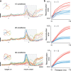
Fig 5. Preferred mode analysis of two control datasets.

The preferred mode is not determined by surface-level features. (a) Analysis for the empirical V1 dataset from Fig 3C and Fig 4A. Shown are three example neurons (left panels) and reconstruction error versus timespan (right panel, reproduced from Fig 3C). (b) Same as in a but the V1 dataset was intentionally manipulated to have structure that was simplest across conditions. (c) Analysis for the empirical M1 dataset from Fig 3E. Shown are three example neurons (left panels) and reconstruction error versus timespan (right panel, reproduced from Fig 3E). (d) Same as in c but the M1 dataset was intentionally manipulated to have structure that was simplest across conditions.

Fig 6. Preferred-mode analysis for non-neural data.

Analysis is shown for ten simulated datasets and two muscle populations. Presentation as in Fig 4. (a) Analysis of simulated M1 populations from the simple tuning model. Two simulated populations (top and bottom) were based on recorded kinematic parameters of two animals (J and N), acquired during the same experimental sessions for which the neural populations are analyzed in Fig 4C. (b) As in a, but M1 populations were simulated based on a more complex tuning model. (c) Analysis of populations of muscle responses (monkeys J and N, top and bottom) recorded using the same task/conditions as in Fig 4D. (d) Analysis of two simulated M1 populations from the dynamical ‘generator model’ that was trained to reproduce patterns of muscle activity. The model was trained to produce the patterns of deltoid activity from the muscle populations in panel c. (e) Analysis of two simulated M1 populations from a neural network model trained to produce the patterns of muscle activity shown in panel c. (f) Analysis of two simulated M1 populations from a ‘non-normal’ neural network model.

Fig 7. Reconstruction error as a function of the number of basis elements.

Each panel plots the difference in reconstruction errors (reconstruction error using k basis-conditions minus reconstruction error using k basis-neurons). The full timespan is considered. Positive values indicate neuron-preferred structure while negative values indicate condition-preferred structure (colored backgrounds for reference). All values in each panel are normalized by a constant, chosen as the smaller of the two reconstruction errors (for the full timespan) plotted in corresponding panels of Figs 4and 6. For most datasets we considered k from 1–20 (mode preference did not flip for higher k in any dataset). For datasets with fewer than 20 neurons (or muscles) values are plotted up to the maximum possible k: the number of neurons (or muscles) in the dataset.

Fig 8. The preferred-mode analysis applied to simulated linear dynamical systems.

Left column of each panel: graphical models corresponding to the different systems. Middle column of each panel: response of neuron 1 in each simulated dataset. Colored traces correspond to different conditions. Right column of each panel: preferred-mode analysis applied to simulated data from that system. Analysis is performed on the data x in panels a-d, while analysis is performed on the data y in panels e-h. (a) A system where inputs u are strong and there are no internal dynamics (i.e., there is no influence of x_t on x_t+1. (b) A system with strong inputs and weak dynamics. (c) A system with weak inputs and strong dynamics. (d) A system with strong dynamics and no inputs other than an input u₀ at time zero that sets the initial state. (e) A system with 20-dimensional linear dynamics at the level of the state x, but where the observed neural responses y reflect only 3 of those dimensions. I.e., the linear function from the state x to the neural recordings y is rank 3. (f) A system with 20-dimensional dynamics and 4 observed dimensions. (g) A system with 20-dimensional dynamics and 8 observed dimensions. (h) A system with 20-dimensional dynamics where all 20 dimensions are observed (formally equivalent to the case in panel d).

Fig 9. Preferred-mode analysis using a variable number of conditions.

(a) Responses of one example neuron illustrating an instance of randomly selected sets of 10 (top), 20 (middle), and 30 (bottom) conditions. Horizontal and vertical calibration bars correspond to 200 ms and 20 spikes/s. (b) Reconstruction error as a function of timespan for sets of 10 (top), 20 (middle), and 30 (bottom) conditions. Multiple traces are shown: one each for 10 draws of random conditions. Dark traces show the neuron-mode (red) and condition-mode (blue) reconstruction error for the particular sets of conditions illustrated in a. Even for small numbers of conditions (as few as 10) there was a consistent preferred mode. In fact, the preferred mode was even more consistent than it appears, as the comparisons are naturally paired: every red trace has a corresponding blue trace. These tended to move upwards and downwards together (as in the example illustrated with the dark traces) with a reasonably consistent difference between them.

Fig 10. Effect of spike filtering width on the preferred mode.

Spike trains from V1 and M1 datasets were filtered with a Gaussian kernel of varying widths (width corresponds to the standard deviation of the Gaussian). (a) Response of one example V1 neuron for filter widths of 10 ms, 20 ms (the default value used for all other analyses in this study), and 100 ms. (b) Response of one example M1 neuron for the same three filter widths. Horizontal and vertical calibration bars correspond to 200 ms and 20 spikes/s. (c) Difference in reconstruction error between the condition mode and the neuron mode (computed as in Fig 7) as a function of filter width, for the V1 dataset from panel a. Differences are positive, indicating that the neuron mode incurred less error and is preferred. Green arrows indicate filter widths of 10, 20, and 100, corresponding to the examples shown in a. (d) Difference in reconstruction error for the M1 dataset from panel b. Differences are negative, indicating that the condition mode incurred less error and is preferred. Thus, the preferred mode is robust to filter width, despite the wide range of frequencies highlighted or suppressed by filter width choices.

References

1. Churchland MM, Shenoy KV. Temporal complexity and heterogeneity of single-neuron activity in premotor and motor cortex. J Neurophysiol. 2007;97: 4235–4257. 10.1152/jn.00095.2007 - DOI - PubMed
1. Raposo D, Kaufman MT, Churchland AK. A category-free neural population supports evolving demands during decision-making. Nat Neurosci. Nature Publishing Group; 2014;17: 1784–1792. 10.1038/nn.3865 - DOI - PMC - PubMed
1. Bair W, Koch C. Temporal precision of spike trains in extrastriate cortex of the behaving macaque monkey. Neural Comput. 1996. - PubMed
1. Benucci A, Ringach DL, Carandini M. Coding of stimulus sequences by population responses in visual cortex. Nat Neurosci. 2009;12: 1317–1324. 10.1038/nn.2398 - DOI - PMC - PubMed
1. Grillner S. Biological pattern generation: the cellular and computational logic of networks in motion. Neuron. 2006;52: 751–766. 10.1016/j.neuron.2006.11.008 - DOI - PubMed
Publication types