Segmentation of 3D Trajectories Acquired by TSUNAMI Microscope: An Application to EGFR Trafficking

Abstract

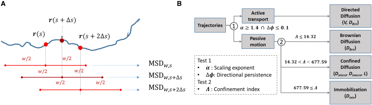
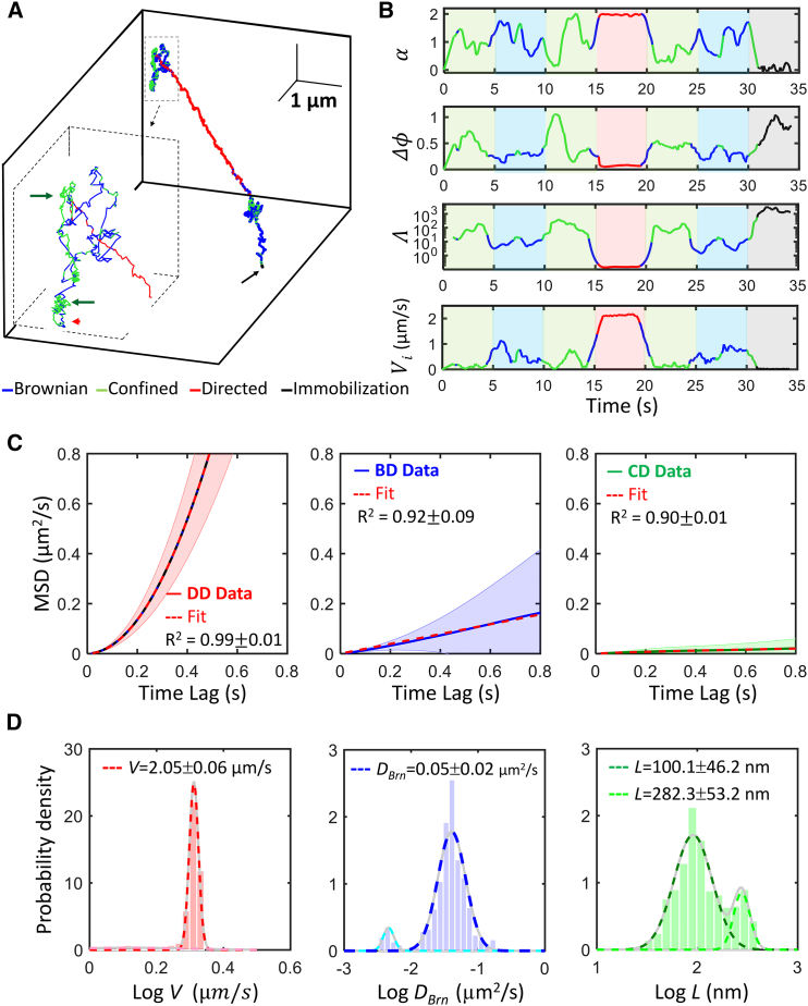
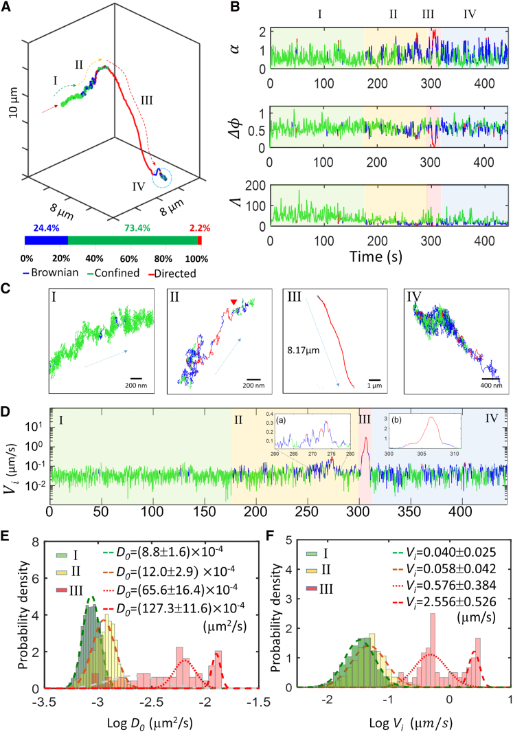
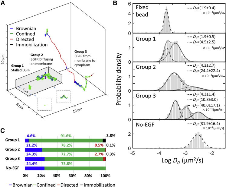
Whereas important discoveries made by single-particle tracking have changed our view of the plasma membrane organization and motor protein dynamics in the past three decades, experimental studies of intracellular processes using single-particle tracking are rather scarce because of the lack of three-dimensional (3D) tracking capacity. In this study we use a newly developed 3D single-particle tracking method termed TSUNAMI (Tracking of Single particles Using Nonlinear And Multiplexed Illumination) to investigate epidermal growth factor receptor (EGFR) trafficking dynamics in live cells at 16/43 nm (xy/z) spatial resolution, with track duration ranging from 2 to 10 min and vertical tracking depth up to tens of microns. To analyze the long 3D trajectories generated by the TSUNAMI microscope, we developed a trajectory analysis algorithm, which reaches 81% segment classification accuracy in control experiments (termed simulated movement experiments). When analyzing 95 EGF-stimulated EGFR trajectories acquired in live skin cancer cells, we find that these trajectories can be separated into three groups-immobilization (24.2%), membrane diffusion only (51.6%), and transport from membrane to cytoplasm (24.2%). When EGFRs are membrane-bound, they show an interchange of Brownian diffusion and confined diffusion. When EGFRs are internalized, transitions from confined diffusion to directed diffusion and from directed diffusion back to confined diffusion are clearly seen. This observation agrees well with the model of clathrin-mediated endocytosis.

Figure 1

Procedure for segmentation and classification of trajectories. (A) The rolling window analysis is conducted at a given time point s with the length of rolling window of 1.6 s (w = 1.6 s) and the sliding time step (Δs) of 0.1 s. (B) The transient behaviors of a trajectory are identified using the three classification parameters: scaling exponent of MSD curve (α), directional persistence (Δϕ), and confinement index (Λ). The MSD curve of each segment is fitted with the proper model to extract the dynamic parameters including V, D_Brn, D_micro, D_macro, L, and D_min. To see this figure in color, go online.

Figure 2

Verifying the trajectory analysis algorithm using SME system (n = 16). (A) A representative prescribed trajectory is composed of Brownian diffusion (BD), confined diffusion (CD), directed diffusion (DD), and immobilization (IM). Simulated conditions are Brownian diffusivity D_pre = 0.08 μm²/s, linear dimension of the confinement L_pre = 100 nm, probability of penetration P = 0.01, and speed of directed diffusion V_pre = 2 μm/s. The track duration is 35 s, and the trajectory is equally divided into seven 5-s-long regions in which the tracked particle exhibits four types of motional modes in the following sequence: CD→BD→CD→DD→CD→BD→IM. The red arrowhead marks the starting point of the trajectory. The green arrows mark the regions exhibiting confined diffusion and the black arrow marks the immobilization region. (B) Time traces of the three classification parameters (α, Δϕ, Λ) and instantaneous velocity (V_i) of the representative trajectory shown in (A). (C) The ensemble-averaged MSD curves from the classified regions were fitted with the proper models to recover the dynamic parameters (D_Brn, L, and V). The R-squared values were employed to evaluate the goodness-of-fit. Ribbons represent the standard deviations. (D) Normalized histograms of experimentally derived dynamic parameters logV (red), logD_Brn (blue), and logL (green) are provided. The means and standard deviations were from curve fitting with a Gaussian mixture model. The total number of trajectories analyzed is 16 in (C) and (D). To see this figure in color, go online.

Figure 3

Interchanging of confined diffusion and Brownian diffusion on cell membrane. (A) A representative trajectory of EGFR membrane diffusion is shown. The green and blue colors represent confined diffusion and Brownian diffusion, respectively. The zoom-in view (inset) shows the membrane confinements based on visual inspection. The fractions of free diffusion time and confinement time were 14.7% and 85.3%, respectively. (B) Time traces of the three motion classification parameters (α, Δϕ, Λ) and instantaneous velocity (V_i) of the representative trajectory shown in (A) are provided. (C) The ensemble-averaged MSD curves from the classified segments were fitted with the proper models to extract D_Brn and L. The R-squared values were employed to evaluate the goodness-of-fit. Ribbons represent the standard deviations. (D) Histograms of logD_Brn and logL derived from the classified segments are provided. These histograms were fitted with a Gaussian mixture model. To see this figure in color, go online.

Figure 4

Trafficking from membrane to cytoplasm. (A) A representative trajectory of EGFR trafficking from cell membrane to cytoplasm is shown. The green, blue, and red colors represent confined, Brownian, and directed diffusion, respectively. The dark red arrow marks the starting point of the trajectory. The fractions of free diffusion time, confinement time, and active transport time were 24.4%, 73.4%, and 2.2%, respectively. The trajectory can be divided into four phases by visual inspection. (B) Time traces of the three motion classification parameters (α, Δϕ, Λ) is shown. Corresponding periods of the four phases are color-coded in these time traces. (C) Zoom-in views of the four phases, which clearly show the differences in the receptor motion in these phases. In this case, EGFR complex traveled 8.17 μm into the cytoplasm at phase III. (D) Time trace of instantaneous velocity (V_i) is shown. A small peak was noted around 273 s in phase II (inset a) and a large peak took place around 307 s in phase III (inset b), which mark the onset of internalization and the motor-mediated transport, respectively. (E) Histograms of logD₀ in phases I–III are provided. (F) Histograms of logV_i in phases I–III are provided. The values shown in (E) and (F) represent the means and standard deviations from Gaussian mixture model fitting. The logD₀ and logV_i of phase III clearly show two distributions. These two distributions are indicated with dotted line and dashed line, respectively. To see this figure in color, go online.

Figure 5

Dividing EGFR trajectories into three groups. (A) 95 EGF-stimulated EGFR trajectories were categorized into three groups that represent stalled EGFRs (group 1, n = 23), membrane-diffusing EGFRs (group 2, n = 49), and membrane-to-cytoplasm-trafficking EGFRs (group 3, n = 23). The inset shows a zoom-in view of the representative trajectories from groups 1 and 2. The trajectories are color-coded to indicate different motional modes within each segment. The dark red arrow marks the starting point of the trajectory of the group 3 representative trajectory. (B) Histograms of logD₀ derived from EGF-stimulated EGFR trajectories (groups 1–3) and the ones without EGF stimulation (No-EGF, n = 15) are provided. These histograms were fitted with a Gaussian mixture model. The detection limit (D_min) is estimated by tracking of fixed beads. (C) Percentages of the four motional modes within the trajectories of the three EGF-stimulated groups and the no-EGF group are provided. To see this figure in color, go online.

References

1. Shera E.B., Seitzinger N.K., Soper S.A. Detection of single fluorescent molecules. Chem. Phys. Lett. 1990;174:553–557.
1. Ambrose W.P., Goodwin P.M., Keller R.A. Single molecule fluorescence spectroscopy at ambient temperature. Chem. Rev. 1999;99:2929–2956. - PubMed
1. Sauer M., Zander C. Single Molecule Detection in Solution. Wiley-VCH Verlag; Hoboken, NJ: 2003. Single molecule identification in solution: Principles and applications; pp. 247–272.
1. Toomre D., Bewersdorf J. A new wave of cellular imaging. Annu. Rev. Cell Dev. Biol. 2010;26:285–314. - PubMed
1. Betzig E., Patterson G.H., Hess H.F. Imaging intracellular fluorescent proteins at nanometer resolution. Science. 2006;313:1642–1645. - PubMed