A study of the synthetic methods and properties of graphenes

Abstract

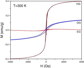
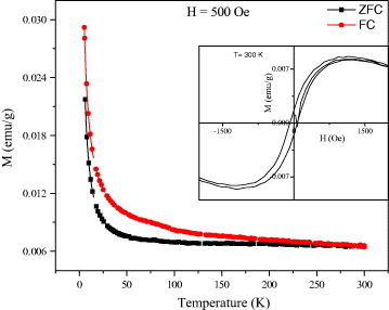
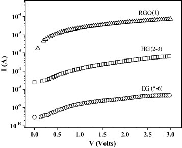
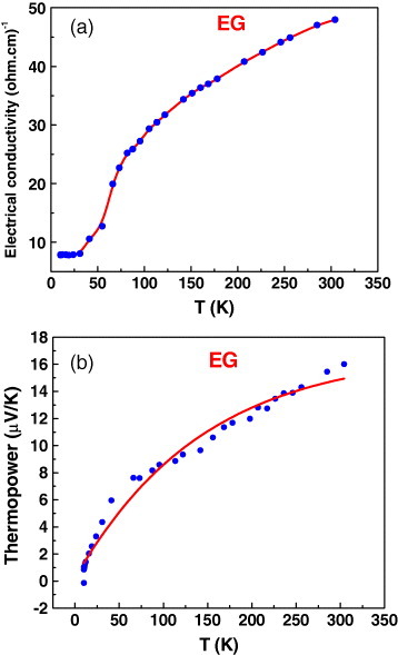
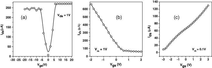
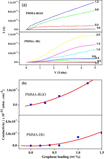
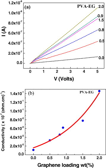
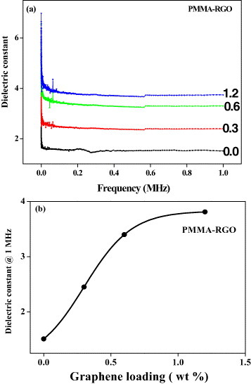
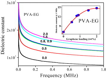
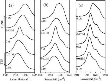
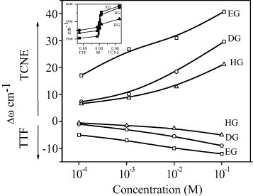
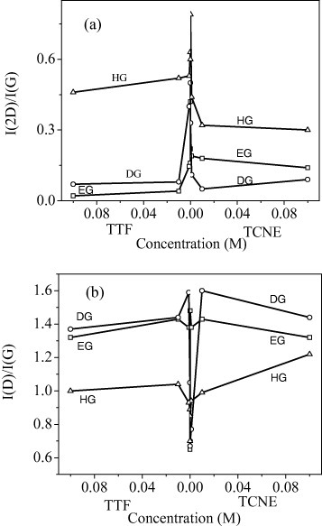
Graphenes with varying number of layers can be synthesized by using different strategies. Thus, single-layer graphene is prepared by micromechanical cleavage, reduction of single-layer graphene oxide, chemical vapor deposition and other methods. Few-layer graphenes are synthesized by conversion of nanodiamond, arc discharge of graphite and other methods. In this article, we briefly overview the various synthetic methods and the surface, magnetic and electrical properties of the produced graphenes. Few-layer graphenes exhibit ferromagnetic features along with antiferromagnetic properties, independent of the method of preparation. Aside from the data on electrical conductivity of graphenes and graphene-polymer composites, we also present the field-effect transistor characteristics of graphenes. Only single-layer reduced graphene oxide exhibits ambipolar properties. The interaction of electron donor and acceptor molecules with few-layer graphene samples is examined in detail.

Keywords: charge-transfer; electronic properties; field-effect transistor characteristics; graphenes; magnetic properties; mechanical properties; preparation methods; surface variations.

Figure 1.

TEM images of graphene prepared by the thermal decomposition of (a, b) methane (70 sccm) and (c) benzene (Ar passed through benzene at a flow rate of 200 sccm), at 1000 ° C on a nickel sheet. Insets in (a) and (c) show electron diffraction patterns from the corresponding graphene sheets.

Figure 2.

Raman spectra of graphene prepared by the thermal decomposition of hydrocarbons on a nickel sheet: (a) methane (70 sccm) at 1000 ° C, (b) ethylene (4 sccm) at 900 ° C, (c) benzene (argon passed through benzene at a flow rate of 200 sccm) at 1000 ° C, (d) benzene (argon passed through benzene at a flow rate of 400 sccm) at 1000 ° C.

Figure 3.

Raman spectra of graphene prepared by the decomposition of (a) methane (64 sccm) at 1000 ° C and (b) acetylene (4 sccm) at 800 ° C on a cobalt sheet.

Figure 4.

TEM images of (a) DG-1650, (b) DG-1850, (c) DG-2050 and (d) DG-2200 samples. The sample number indicates the temperature of transformation in ° C.

Figure 5.

Histograms of height profile and lateral dimensions of (a) DG-1650 and (b) DG-2200 samples obtained from the analysis of AFM images.

Figure 6.

Raman spectra of (a) DG-1600 and (b) DG-2200 samples.

Figure 7.

(a) TEM and (b) AFM images of HG material prepared by arc discharge of graphite in hydrogen. (Reproduced with permission from [4] © 2010 American Chemical Society.)

Figure 8.

Temperature dependence of magnetization of EG sample at 500 Oe and 1 T. (Reproduced with permission from [46] © 2009 American Chemical Society.)

Figure 9.

Magnetic hysteresis in EG, DG and HG samples at 300 K. (Reproduced with permission from [46] © 2009 American Chemical Society.)

Figure 10.

Temperature variation of magnetization of EGH (W) at 500 Oe showing the ZFC and FC data. The inset shows the magnetic hysteresis at 300 K. EGH (W) stands for graphene prepared by exfoliation of graphene oxide followed by hydrazine reduction with prior washing with 8-hydroxy-quinoline-5-sulfonic acid.

Figure 11.

FESEM images of a platinum thin-film electrode separated by 70 nm, without any graphene sample (a), and with different graphene samples that were drop cast between the gap, namely, RGO (b), HG (c) and EG (d).

Figure 12.

I–V characteristics of RGO, HG and EG samples (the number of layers is shown in parenthesis).

Figure 13.

Temperature variations of (a) electrical conductivity and (b) thermopower for an EG sample.

Figure 14.

Transfer characteristics (I_ds versus V_gs) of FETs based on (a) RGO, (b) B-HG and (c) N-HG. Here, I_ds, V_ds and V_gs stand for source to drain current, source to drain voltage and gate to source voltage, respectively. (Reproduced with permission from [60] © 2010 Elsevier B. V.)

Figure 15.

(a) I–V characteristics of PMMA composites with different percentages of RGO and HG. (b) Electrical conductivity as a function of graphene nanofiller loadings (wt%) for PMMA composites with RGO and HG.

Figure 16.

(a) I–V characteristics of PVA-EG graphene composites for various nanofiller loading. (b) Electrical conductivity as a function of graphene nanofiller loadings (wt%) for PVA-EG composites with acid-functionalized EG.

Figure 17.

(a) Variation of dielectric function of PMMA-RGO composites with frequency for various nanofiller contents (wt%). (b) Dielectric function (at 1 MHz) as a function of graphene loading (wt%) for PMMA-RGO graphene composites.

Figure 18.

Variation of dielectric function with frequency for PVA-EG graphene composites having various nanofiller contents. The inset shows the dielectric function (at 1 MHz) as a function of loading (wt%) for PVA composites with acid-functionalized EG.

Figure 19.

Variation in the Raman G-bands of graphene samples (a) EG, (b) DG and (c) HG, caused by interaction with varying concentrations of TTF and TCNE. (Reproduced with permission from [67] © 2009 Elsevier B. V.)

Figure 20.

Changes in the G-band position plotted against the logarithm of concentration of TTF or TCNE. The inset shows a linear plot against the concentration. (Reproduced with permission from [67] © 2009 Elsevier B. V.)

Figure 21.

Variation in the (a) 2D/G and (b) D/G intensity ratios with the concentration of TTF and TCNE. (Reproduced with permission from [67] © 2009 Elsevier B. V.)

References

1. Geim A K. and Novoselov K S. Nat. Mater. 2007;6:183. doi: 10.1038/nmat1849. - DOI - PubMed
1. Rao C N R, Sood A K, Subrahmanyam K S. and Govindaraj A. Angew. Chem. Int. Ed. 2009;48:7752. doi: 10.1002/anie.200901678. - DOI - PubMed
1. Geim A K. Science. 2009;324:1530. doi: 10.1126/science.1158877. - DOI - PubMed
1. Rao C N R, Sood A K, Voggu R. and Subrahmanyam K S. J. Phys. Chem. Lett. 2010;1:572. doi: 10.1021/jz9004174. - DOI
1. Allen M J, Tung V C. and Kaner R B. Chem. Rev. 2009;110:132. doi: 10.1021/cr900070d. - DOI - PubMed
LinkOut - more resources