Parameter set for computer-assisted texture analysis of fetal brain

Abstract

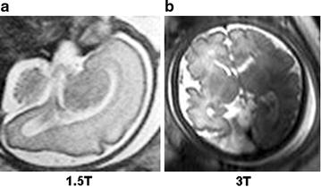
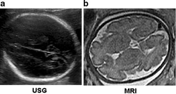
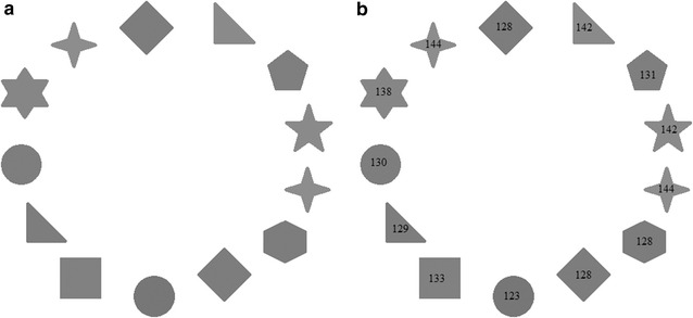
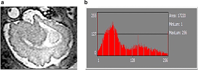
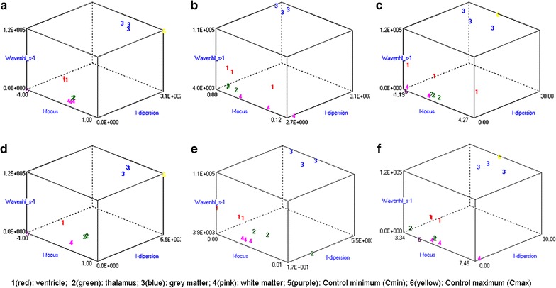
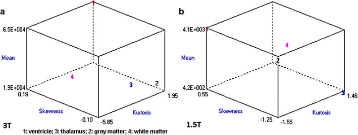
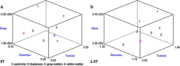
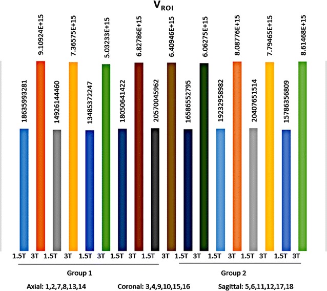
Background: Magnetic resonance data were collected from a diverse population of gravid women to objectively compare the quality of 1.5-tesla (1.5 T) versus 3-T magnetic resonance imaging of the developing human brain. MaZda and B11 computational-visual cognition tools were used to process 2D images. We proposed a wavelet-based parameter and two novel histogram-based parameters for Fisher texture analysis in three-dimensional space.

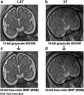
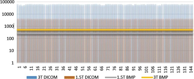
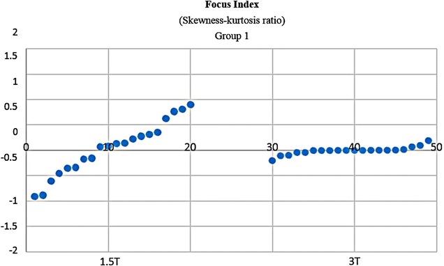
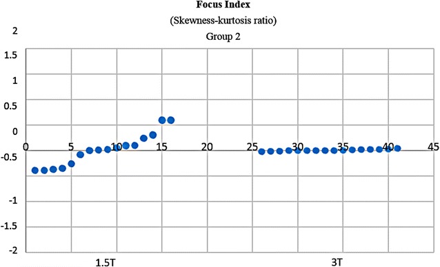
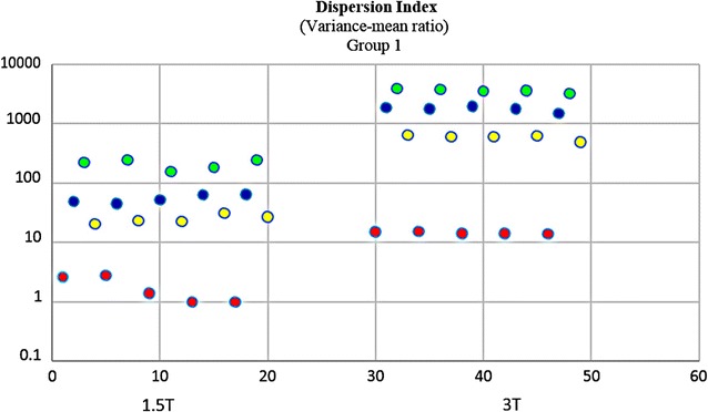
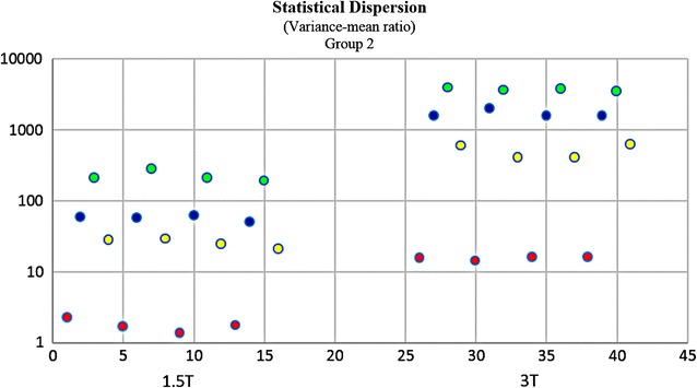
Results: Wavenhl, focus index, and dispersion index revealed better quality for 3 T. Though both 1.5 and 3 T images were 16-bit DICOM encoded, nearly 16 and 12 usable bits were measured in 3 and 1.5 T images, respectively. The four-bit padding observed in 1.5 T K-space encoding mimics noise by adding illusionistic details, which are not really part of the image. In contrast, zero-bit padding in 3 T provides space for storing more details and increases the likelihood of noise but as well as edges, which in turn are very crucial for differentiation of closely related anatomical structures.

Conclusions: Both encoding modes are possible with both units, but higher 3 T resolution is the main difference. It contributes to higher perceived and available dynamic range. Apart from surprisingly larger Fisher coefficient, no significant difference was observed when testing was conducted with down-converted 8-bit BMP images.

Keywords: Artificial intelligence; Computational visual cognition; Computer-assisted radiology; Fetal brain; Histogram; Hugues Gentillon; Mazda; Medical cybernetics; Prenatal development; Teleradiology; Wavelets; b11.

Fig. 1

“Do you see what I see?”. Fetal brain. a Left 1.5 T. b Right 3 T. This figure was incorporated and so-titled in this manuscript to illustrate that magnetic resonance (MR) images can be used for evaluation of achromatic vision and sensitivity to change in grayscale quality between different subjects. For fair comparison, this exercise should be blinded. It is recommended to have at least two radiologists, if not available, medically-trained practitioners or any volunteers (blinded) and one examiner (also blinded) to look at the images side-by-side, on two medical-diagnostic monitors, engineered for 16-bit display (same brand/model in natively flat display mode: i.e. without any added enhancements). All in-computer/in-monitor RT (real-time) editing features must be turned off (incl. hardware/software rendering): n.b. 16-bit of true data has more room for “contrast booster”—which is essentially an illusion, as a result of post-editing artifacts, not really part of the image. In this investigation, volunteers were asked to identify the images unlabeled (, of course). It was observed that both images were equally sharp (in pass-through mode), for a normal, naked human eye. There flows the explanation for the research goal to mathematically determine which MR modality actually produces images with more captured details. Both images were 16-bit encoded, and the difference could not be measured via “perceived dynamic range” (visible details). With computer vision software, 1.5/3 T images can be numerically decoded to accurately assess “available dynamic range” (visible/invisible details)

Fig. 2

Ultrasonography (USG) vs. magnetic resonance imaging (MRI). Fetal MRI was used as a complimentary modality to USG. a USG. b MRI

Fig. 3

Varying shades of grey. a Arrange from lighter to darker? b Answers to Puzzle as per measurements from computer vision software. Again, test subjects should be blinded

Fig. 4

Histogram representation of fetal brain. a MRI of fetal brain. b Histogram of the whole image

Fig. 5

Regions of interest. a ROI 1 ventricles; 2 thalamus; 3 grey matter; 4 white matter. b Histogram parameters from texture analysis with MaZda

Fig. 6

ROI analysis. a ROI 1 Ventricles; b ROI 2 Thalamic nuclei; c ROI 3 Grey matter; d ROI 4 White matter. There exist several techniques and methods of texture analysis. Non-parametric graphs (e.g. histogram, box plot) would be indeed a simple alternative to conduct this study. As shown in the figures, MaZda does display histogram of 8-bit but not for 16-bit DICOM image. Also, there are issues with drawing conclusions straight from histograms and boxplots. They are pictorial representations and thus are indirect methods. Furthermore non-parametric interpretation may not be as precise and accurate as parametric quantification. Therefore, parametric quantification was used to assess image quality rather than conventional appearance. 3D, non-parametric graphs are also possible with collateral usage of MaZda (version 5) and B11 (version 3.3) in training mode. The problem with training methods is that errors might occur as a result of overtraining the network. Hence, raw analysis was performed

Fig. 7

a 1.5 T MR image of a fetal brain: 12-bit DICOM format, coronal section. b 3 T MR image of a different subject: 16-bit DICOM, coronal plane. c Same image shown in “a” after conversion to BMP. d Same image shown in “b” after conversion to BMP

Fig. 8

Measured usable bits (pixel values). 3/1.5 T BMP ≈ 256; 1.5 T DICOM ≈ 4096; 3 T DICOM ≈ 65,536

Fig. 9

Graph showing difference between ROIs. Raw-data analysis was performed to compute F with 1-nearest-neighbor (NN) classification and no feature standardization. Same samples and ROIs were used in both pre- and post- image compression. a 1.5 T uncompressed DICOM; Fisher coefficient computation with controls: Cmin = (0, −1, 0); Cmax = (307, 1, 120,000); F = 426.0; MDE = 0%. b Same 1.5 T samples: zoomed in, mostly on the y-axis. c same 1.5 T after compression to 8 bits; Fisher coefficient computation with controls: Cmin = (0, −1, 0) Cmax = (30, 1, 120,000); F = 776.0; MDE = 5.56%. d 3 T uncompressed DICOM: F = 1787.0; MDE = 0%. e Same 1.5 T samples: zoomed in, mostly on the y-axis. f Same 3 T after compression to 8 bits. 3 T: F = 2344.3; MDE = 0%

Fig. 10

a Difference between ROIs for 3 T with two images from same T2 sequence (same patient). 1 ventricle; 3 thalamus; 2 grey matter; 4 white matter. b Difference between ROIs for 1.5 T with two images from same T2 sequence (same patient). 1 ventricle; 3 thalamus; 2 grey matter; 4 white matter

Fig. 11

a Difference between ROIs for 3 T with two images from different T2 TSE [Turbo spin echo sequences (different patients)]. 1 ventricle; 3 thalamus; 2 grey matter; 4 white matter. b Difference between ROIs for 1.5 T with one image from PD and one from T2 HASTE sequence (different patient). 1 ventricle; 3 thalamus; 2 grey matter; 4 white matter

Fig. 12

ROI variability graph showing difference between 1.5 and 3 T

Fig. 13

Sharpness distribution: Group 1 acceptable range is [+1, −1]. Zero is absolute sharpness; in other words, better focus. 3 T has more points closer to zero

Fig. 14

Sharpness distribution: Group 2 acceptable range is [+1, −1]. Zero is absolute sharpness; in other words, better focus. 3 T has more points closer to zero

Fig. 15

Statistical dispersion: logarithmic graph (Group 1) showing difference between 1.5 and 3 T. 3 T ROIs are more spread out; thus better for distinguishing close anatomical structures in fetal MRI. Regions of interest—red: ventricle—yellow: white matter—blue: thalamus—green: grey matter

Fig. 16

Statistical dispersion: logarithmic graph (Group 1) showing difference between 1.5 and 3 T. 3 T ROIs are more spread out; thus better for distinguishing close anatomical structures in fetal MRI. Regions of interest—red: ventricle—yellow: white matter—blue: thalamus—green: grey matter

References

1. Hellman LM, Duffus GM, Donald I, Sunden B. Safety of diagnostic ultrasound in obstetrics. Obstet Gynecol Surv. 1971;26(1):13–14. doi: 10.1097/00006254-197101000-00006. - DOI - PubMed
1. Richards DS. Prenatal ultrasound to detect fetal anomalies. NeoReviews. 2012;13(1):e9–e19. doi: 10.1542/neo.13-1-e9. - DOI
1. Nishi T, Iwasaki M, Yamoto M, Nakano R. Prenatal diagnosis of autosomal recessive polycystic kidney disease by ultrasonography and magnetic resonance imaging. Acta Obstet Gynecol Scand. 1991;70(7–8):615–617. doi: 10.3109/00016349109007927. - DOI - PubMed
1. Kawabata I, Takahashi Y, Iwagaki S, Tamaya T. MRI during pregnancy. J Perinat Med. 2003;31(6):449–458. doi: 10.1515/JPM.2003.070. - DOI - PubMed
1. Bulas D, Egloff A. Benefits and risks of MRI in pregnancy. Semin Perinatol. 2013;37(5):301–304. doi: 10.1053/j.semperi.2013.06.005. - DOI - PubMed
Publication types