Synthetic biology routes to bio-artificial intelligence

Abstract

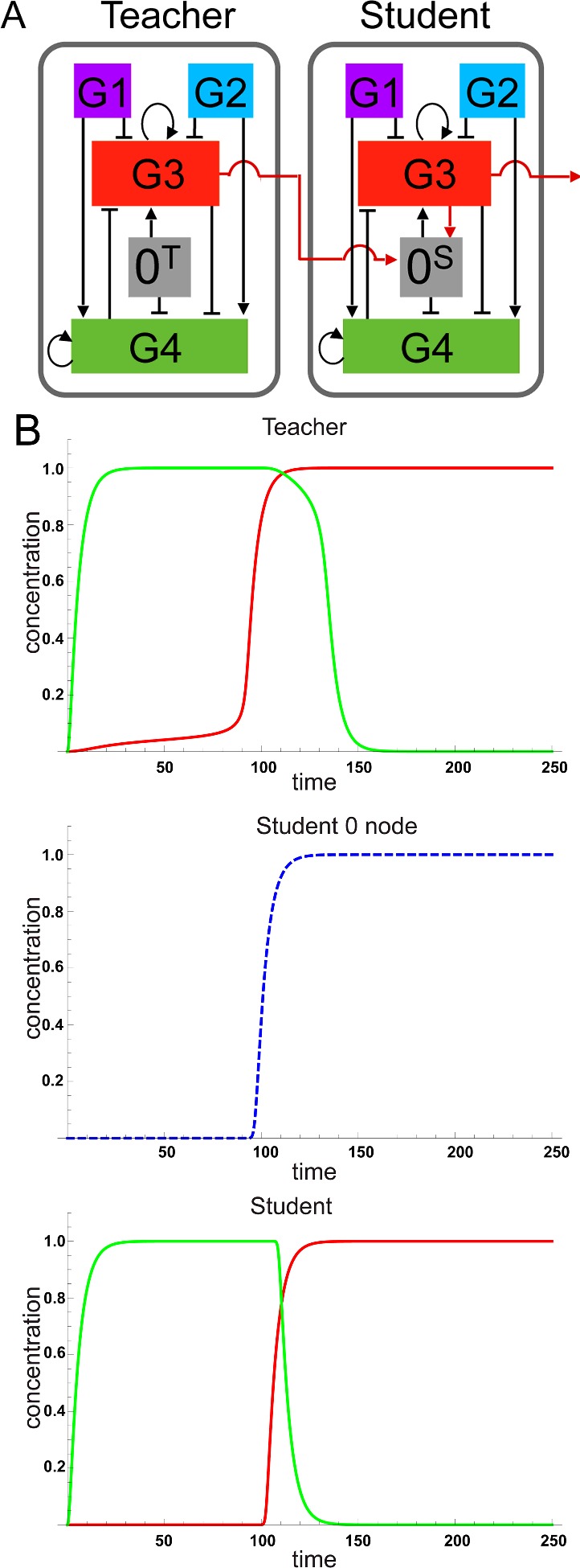
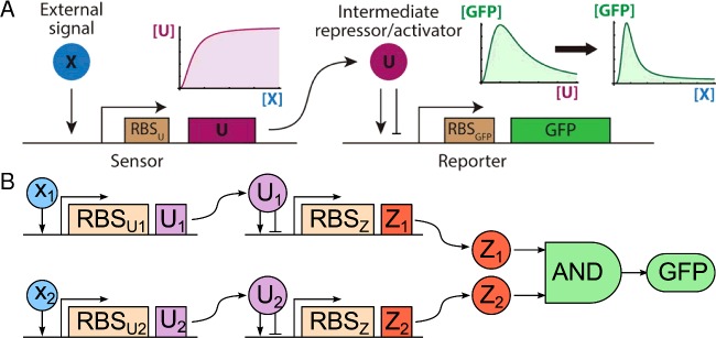
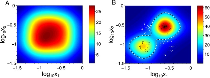
The design of synthetic gene networks (SGNs) has advanced to the extent that novel genetic circuits are now being tested for their ability to recapitulate archetypal learning behaviours first defined in the fields of machine and animal learning. Here, we discuss the biological implementation of a perceptron algorithm for linear classification of input data. An expansion of this biological design that encompasses cellular 'teachers' and 'students' is also examined. We also discuss implementation of Pavlovian associative learning using SGNs and present an example of such a scheme and in silico simulation of its performance. In addition to designed SGNs, we also consider the option to establish conditions in which a population of SGNs can evolve diversity in order to better contend with complex input data. Finally, we compare recent ethical concerns in the field of artificial intelligence (AI) and the future challenges raised by bio-artificial intelligence (BI).

Keywords: artificial intelligence; gene networks; synthetic biological circuits; synthetic biology.

Figure 1. A synthetic gene network for linear classification

A linear classifier phenotype can be achieved with a SGN comprising five nodes, depicted in the diagram as circles labelled 0, 1, 2, 3 and 4. Arrowhead connectors indicate activation of one node by another, hammerhead connectors indicate inhibition. Nodes 3 and 4 represent a toggle switch, which can flip between the state of ‘3 ON, 4 OFF’ and the state of ‘3 OFF, 4 ON’. Nodes 3 and 4 repress each other. Node 0 favours the ‘4 ON’ state and inhibits the ‘3 ON’ state. Nodes 1 and 2 represent inputs that favour ‘3 ON’ and inhibit ‘4 ON’. The output position of the 3/4 toggle switch is tipped toward ‘3 ON’ or ‘4 ON’ depending on the net activity level of nodes 1 and 2. In effect the 3/4 toggle switch classifies inputs 1 and 2. Node 0 can be used to tip the equilibrium of the toggle switch toward ‘3 ON’. This impacts how the output position of the toggle switch is influenced by nodes 1 and 2. In this way, the weighting of the classification threshold can be set by the activity of node 0. This scheme is proposed here by A.Z.

Figure 2. Linear classification with a biological student–teacher network

(A) Teacher and student cells both contain SGNs encoding the five nodes described in Figure 1, but labelled here as 0, G1, G2, G3 and G4. Node 0 for a teacher cell is labelled 0^T and node 0 for a student cell is labelled 0^S. As in Figure 1, nodes G3 and G4 comprise a toggle switch. The output position of the toggle switch is tipped toward G3, resulting in RFP expression or G4, resulting in GFP expression, depending on the net activity level of nodes G1 and G2. In effect the G3/G4 toggle switch classifies the activities of the G1 and G2 nodes as inputs. As in Figure 1, node 0 (0^T or 0^S) pushes the equilibrium of the toggle switch toward G3. Unlike in Figure 1, in this BST network, activity of 0^T can be controlled exogenously by addition of a small molecule inducer to the growth medium. Furthermore, in addition to RFP, node G3 also directs expression of a small molecule that can traverse cell membranes and activate node 0^S. This has the effect that, when teacher cells are in excess, the activity of 0^S in student cells is set (‘learned’) by the level of signal produced by teacher cells. Arrowhead connectors indicate activation of one node by another and hammerhead connectors indicate inhibition. Curled arrowhead connectors indicate auto-induction. (B) Mathematical simulation of the BST network learning dynamics. Outputs of the student cells: red for RFP from G3, green for GFP from G4, are constantly ‘learned’ from changes in the teacher cells which determine the activity (threshold) of node 0^S in the student cells. This scheme is proposed here by A.Z. and D.N. and the simulation was performed by C.G. and Y.S.

Figure 3. Genetic memory circuits

(A) Genetic toggle switch. A sufficiently strong pulse of input 1 will overcome inhibition of expression of gene X caused by protein Y (Y in blue oval). Uninhibited expression of gene X will then continue as protein X (X in blue oval) also acts to inhibit expression of gene Y. Subsequently, the network can be flipped to the opposite position by a sufficiently strong pulse of input 2, which will overcome inhibition of expression of gene Y caused by protein X. Uninhibited expression of gene Y will then continue as protein Y also acts to inhibit expression of gene X. (B) Positive feedback loop circuit. Input 1 initiates expression of gene X. The resultant protein X then also induces express of gene X for sustained activity of the gene that will persist after the initial input 1 has ceased. Positive and negative regulations are indicated by arrows and hammerheads, respectively. These schemes have been proposed by several groups.

Figure 4. A synthetic gene network for associative learning

(A) Schematic diagram of the PFNM associative learning network. Positive and negative regulations are indicated by arrows and hammerheads, respectively. Input 1 stimulates nodes u, v and y. Input 2 stimulates nodes w and y. (B) Simulation of the behaviour of the network. Either input 1 or 2 alone leads to a weak activation of the output y, at times t1 and t2. When both inputs 1 and 2 are applied simultaneously, a ‘memory’ is formed by a self-sustained expression of u due to its positive auto-regulation. Because of this memory a subsequent input 1 or input 2 alone can cause a strong induction of y. In this way the network has learned to associate inputs 1 and 2. This memory can be erased by a sufficiently large input 1 (due to the direct activation of v), bringing the system back to the default state. This scheme is proposed here by Y.S. and M.C.R. and the simulation was performed by Y.S.

Figure 5. SGNs to classify input data that are not linearly separable

(A) Sensing and response functionalities are split into separate modules. In the first module (sensor), an inducible promoter drives the expression of the transcription factor U in response to the concentration of a biological input X, such as a solute or signalling molecule. Above a certain level of X, the expression of U reaches a maximum and does not increase or decrease. In the second module (reporter), another inducible promoter drives the expression of a reporter (GFP) in response to induction by U. The promoter is activated by intermediate concentrations of U and inhibited by high concentrations of U. Thus, the resulting response function of the entire two-promoter circuit to the concentration of signalling molecule is bell shaped for the relevant values of the input signal. (B) In the case of two input ranges, X₁ and X₂, the sensor/output modules feed into an AND gate which sums the output signals as either the presence or absence of GFP expression [30,33]. Adapted with permission from Dydovik et al. [30] and Kanakov et al. [33].

Figure 6. Simulation of an ensemble SGN soft learning how to classify overlapping input signals

(A) The signals from two inputs, X₁ and X₂, overlap and therefore result in production of an overlapping output (red region) from an untrained ensemble SGN population. (B) After such a population has undergone loss of certain cells (indicated by white dots) due to selection pressure, mathematical modelling by Kanakov et al. [33] predicts that a classification border (within black and white dashed line) will emerge in respect to the output signal from the remaining cells (black dots). These remaining cells, and the ensemble of SGNs they harbour, can be considered as a ‘trained classifier’, which has undergone ‘soft learning’. The colour code of the heat map indicate relative change in response of the ensemble classifier, in arbitrary units. Adapted with permission from Kanakov et al. [33].

References

1. Ghahramani Z. Probabilistic machine learning and artificial intelligence. Nature. 2015;521:452–459. doi: 10.1038/nature14541. - DOI - PubMed
1. Nakagaki T., Yamada H., Toth A. Maze-solving by an amoeboid organism. Nature. 2000;407:470. doi: 10.1038/35035159. - DOI - PubMed
1. Tero A., Takagi S., Saigusa T., Ito K., Bebber D.P., Fricker M.D., et al. Rules for biologically inspired adaptive network design. Science. 2010;327:439–442. doi: 10.1126/science.1177894. - DOI - PubMed
1. Saigusa T., Tero A., Nakagaki T., Kuramoto Y. Amoebae anticipate periodic events. Phys. Rev. Lett. 2008;100:018101. doi: 10.1103/PhysRevLett.100.018101. - DOI - PubMed
1. Mangan S., Alon U. Structure and function of the feed-forward loop network motif. Proc. Natl. Acad. Sci. 2003;100:11980–11985. doi: 10.1073/pnas.2133841100. - DOI - PMC - PubMed
Publication types