Computational principles and models of multisensory integration

Abstract

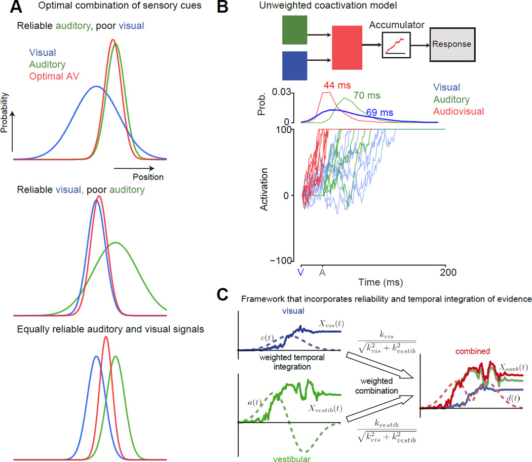
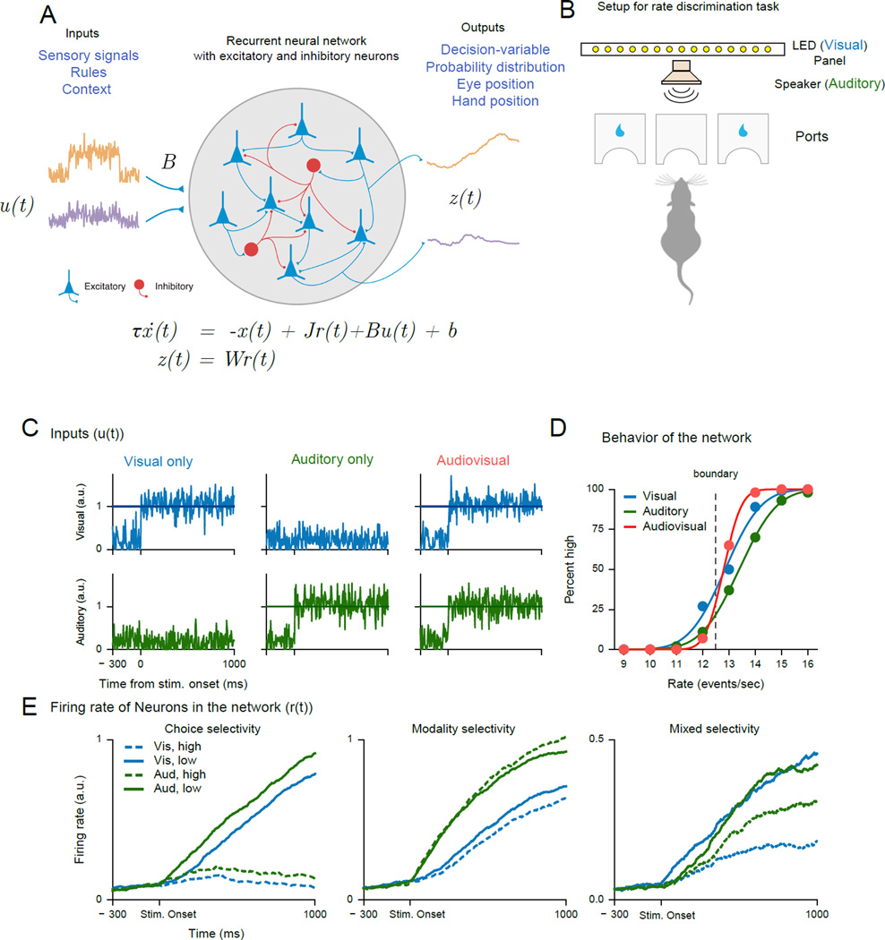
Combining information from multiple senses creates robust percepts, speeds up responses, enhances learning, and improves detection, discrimination, and recognition. In this review, I discuss computational models and principles that provide insight into how this process of multisensory integration occurs at the behavioral and neural level. My initial focus is on drift-diffusion and Bayesian models that can predict behavior in multisensory contexts. I then highlight how recent neurophysiological and perturbation experiments provide evidence for a distributed redundant network for multisensory integration. I also emphasize studies which show that task-relevant variables in multisensory contexts are distributed in heterogeneous neural populations. Finally, I describe dimensionality reduction methods and recurrent neural network models that may help decipher heterogeneous neural populations involved in multisensory integration.

Fig 1. Bayesian frameworks and coactivation models to understand multisensory behavior

A: Near-optimal cue (or stimulus) combination according to the Bayesian framework to improve discrimination behavior is well understood with an example (adapted from [92]). Consider a cat seeking a mouse with both visual and auditory cues. The curves in the figure show the hypothetical probability distributions of the mouse’s position as estimated by the cat’s brain for the three different modalities (Blue-visual, green-auditory, red-audiovisual). Assume that it is dark, and the mouse is in an environment with many gray rocks roughly the size and shape of a mouse. In this context, the optimal Bayesian cat would use auditory cues to estimate the mouse’s location (top). In contrast, when it is sunny, to optimize its discrimination behavior the cat would largely rely on visual cues to locate the mouse (middle). One can readily imagine many intermediate scenarios where the optimal strategy for the cat is to combine both visual and auditory cues to have the best chance of catching the mouse (bottom). For the case that the cat’s auditory and visually guided estimates of the mouse’s position are Gaussian, independent and unbiased (means: s_a, s_v and standard deviations σ_a, σ_v ), the optimal estimate of the position of the mouse is the weighted average of the auditory and visually guided estimates (S_av = W_aS_a+W_vS_v). The weights are the normalized reliability of each cue ($W_a=\frac{\frac{1}{{\sigma }_a^2}}{\frac{1}{{\sigma }_a^2}+\frac{1}{{\sigma }_v^2}},W_v=\frac{\frac{1}{{\sigma }_v^2}}{\frac{1}{{\sigma }_a^2}+\frac{1}{{\sigma }_v^2}}$). Behavior in multisensory discrimination experiments can be tested to see if they are consistent with this prediction from the optimal framework. B: An example of a simple coactivation model used to explain detection behavior. Top panel, a cartoon of the linear summation coactivation model typically used to explain multisensory detection behavior [46,47]. Auditory and visual inputs are linearly summed to arrive at a new drift-rate, and this undergoes the drift-diffusion process to the criterion to trigger a response. Bottom panel, simulations from the coactivation model of a few trials of an audiovisual stimulus where a visual cue turns on at t=0 and an auditory cue turns on at t=30 ms. The visual and the auditory stimuli were assumed to be modest in intensity. In this hypothetical integrator, the onset of the visual stimulus before the onset of the auditory stimulus results in an increase in activity. The auditory stimulus can build on this activity, and this results in the criterion being reached faster on average for the audiovisual (44 ms) compared to both auditory (~70 ms RT when measured relative to the visual stimulus onset) and visual-only stimuli (~69 ms). Blue lines denote the visual cue. The green lines denote the auditory cue. Red lines denote the audiovisual cue. C: A framework that combined the insights from both A and B to develop an optimal coactivation drift-diffusion model to explain multisensory discrimination behavior [48]. This model was developed in the context of a heading discrimination task using both visual and vestibular cues. The key innovation in this model is that it integrates evidence in an optimal manner by factoring in the model both the time course of sensory signals as well as the reliability of the signals. The visual and vestibular cues are time varying signals, whose reliabilities change as a function of time. They also can have different reliabilities depending on the context (as in A). Simply adding as in B is suboptimal. For instance, you would just be adding noise at the start when the visual signal is low. X_vis(t) = integrated evidence for the visual cue (optic flow), X_vest (t) is the integrated evidence for the vestibular cue. k_vis is a constant that signifies the strength of the visual signal. k_vestib is a constant that signifies the strength of the vestibular signal. The combined signal X_comb (t)is the reliability-weighted sum of these two signals (weights are shown on top of the arrows). The dashed lines on the left-hand side of the figure denote the velocity and acceleration profiles of the signals. The velocity profile was Gaussian. Both visual and vestibular cues were presented congruently and were temporally synchronized. In this study, momentary evidence for vestibular input is assumed to result from acceleration (a(t)). The momentary evidence for visual input is thought to result from velocity cues (v(t)).

Fig. 2. Simulations from the RNN model developed in Song et. al. [90] to solve the multisensory integration task reported in Raposo et al. [87]

A: A schematic and dynamical equation for a nonlinear RNN. x(t) is a vector with the i^th component of this vector describing the summed and filtered synaptic current input for the i^th neuron (as in a biological neuron). The continuous variable r (t) is a vector and describes the FR of neurons in the network and are obtained through a nonlinear transform of x(t), typically a saturating nonlinearity or a rectified linear function. The defining feature of these RNNs is the recurrent feedback from one neuron in the network to another. The matrix J parameterizes the connection strength between the units. The network receives external input through the u(t) term weighted by a vector B; every neuron also receives a bias input b_i. τis a time constant that sets the time scale of the network. The outputs of the network, z(t), are usually obtained by a linear readout operation. Each node in this network is a neuron that receives external input as well as recurrent feedback (through J). Inputs (u(t)) can be sensory signals, rules, or context signals. The outputs (z(t)), which are obtained by a weighted readout of the firing rates of the neurons in the network can be binary choice [75], continuous decision-variables, probability distributions, or behavioral signals such as hand position/eye position[90]/electromyography responses [89]. The RNN cartoon is adapted from Fig. 1 of [90]. B: Schematic of the behavioral apparatus for the multisensory rate discrimination task for the rats in [87] (redrawn based on Fig. 1A in [87]). The Stimuli were 1s long auditory and/or visual streams delivered either through a speaker or from a LED panel. The rats discriminated whether the presented rate was lower (move to left port) or higher (move to right port) than a decision boundary (12.5 events/sec). The rat cartoon is a recolored version of the one in Fig. 1A of [87]. C: Inputs to a model network trained to solve the audiovisual integration task from [87]. The network was trained to perform the same task and provided with both positive and negatively tuned visual and auditory input ( u(t), positive inputs are shown here). The RNN consisted of 150 neurons (120 Excitatory and 30 inhibitory) and used a rectified linear current (x(t)) to firing rate (r(t)) function. The network was trained to hold a high output value if the input was above the decision boundary (12.5 events/sec) and low if the input was below this decision-boundary. The results shown were obtained from the code provided in [90] (https://github.com/frsong/pycog) D: The RNN solves the task and shows a benefit for multisensory compared to unisensory stimuli and thus demonstrates behavior similar to the rats in the original study [87]. The psychometric functions show the percentage of high choices made by the network as a function of the event rate for the uni- and multisensory trials. The smooth lines are cumulative Gaussian fits to the psychometric function. E: FR (r(t)) of selected simulated neurons in the RNN aligned to the stimulus onset during the period of sensory stimulation and decision-formation. In particular, some neuronal FRs show the main effect of choice (left panel); FRs of other neurons show a main effect for modality (middle panel). Also as in the real data recorded in the posterior parietal cortex [87], neurons demonstrate FRs best described by an interaction between choice and modality tuning (right panel). High and low denote the choices. Vis-high denotes that the rats chose high for the visual input for example and so on.

References

1. Ernst MO, Bulthoff HH. Merging the senses into a robust percept. Trends in Cognitive Sciences. 2004;8:162–169. - PubMed
1. Spence C. Multisensory Flavor Perception. Cell. 2015;161:24–35. - PubMed
1. Maier JX, Blankenship ML, Li JX, Katz DB. A Multisensory Network for Olfactory Processing. Curr Biol. 2015;25:2642–2650. - PMC - PubMed
1. Alais D, Newell FN, Mamassian P. Multisensory processing in review: from physiology to behaviour. Seeing Perceiving. 2010;23:3–38. - PubMed
1. Chandrasekaran C, Trubanova A, Stillittano S, Caplier A, Ghazanfar AA. The natural statistics of audiovisual speech. PLoS Comput Biol. 2009;5:e1000436. - PMC - PubMed
LinkOut - more resources