climwin: An R Toolbox for Climate Window Analysis

Abstract

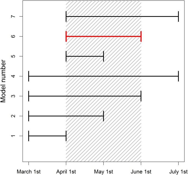
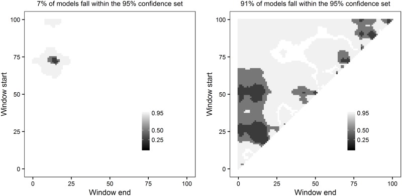
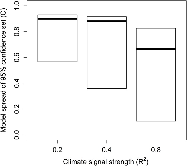
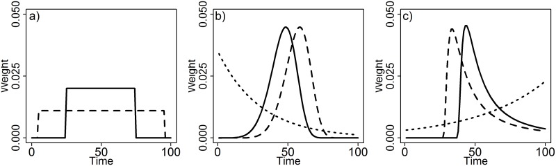
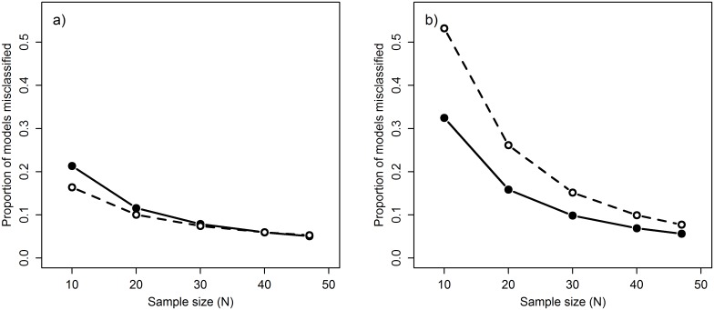
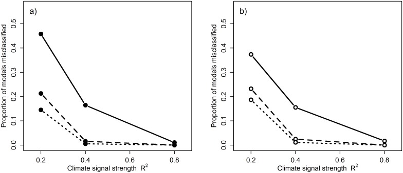
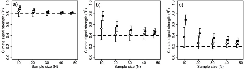
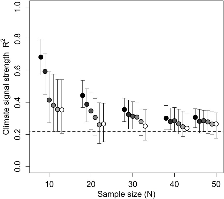
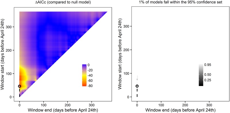
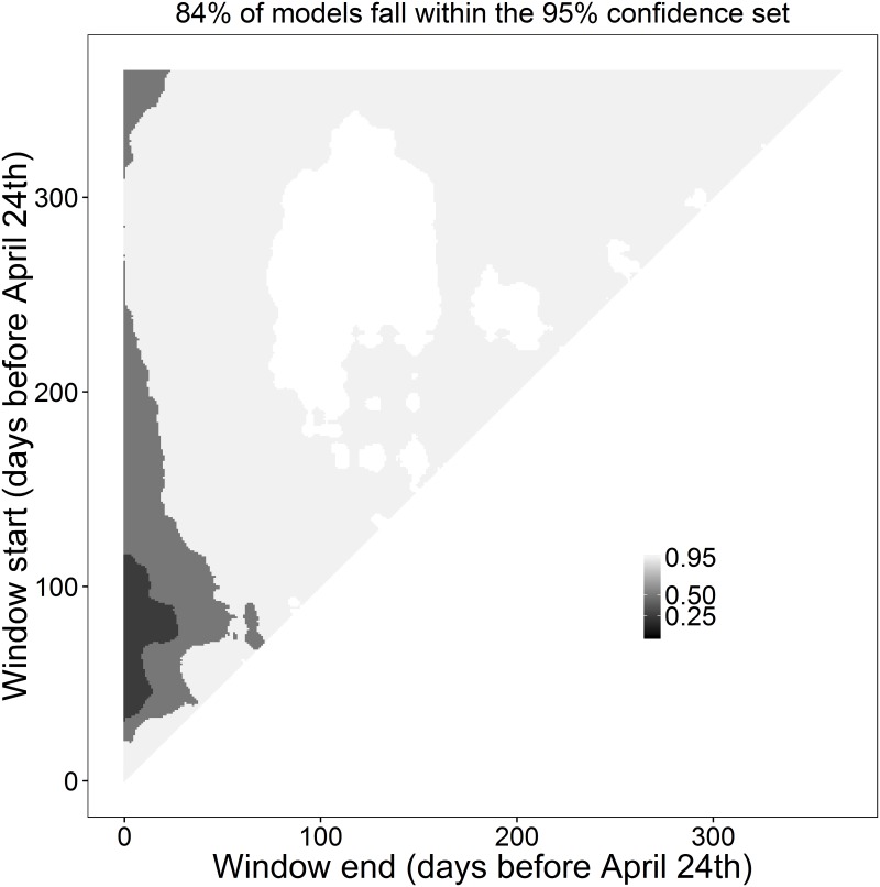
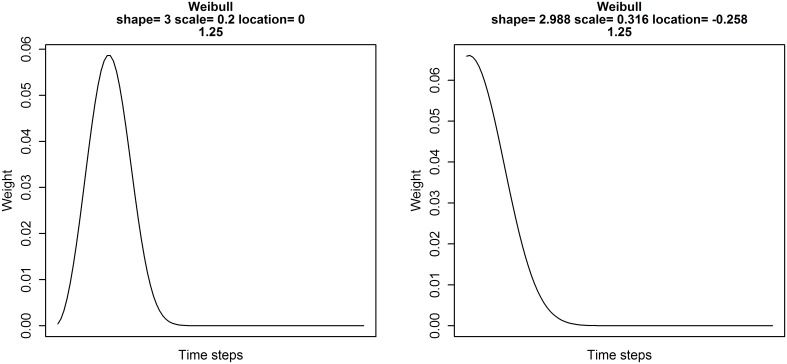
When studying the impacts of climate change, there is a tendency to select climate data from a small set of arbitrary time periods or climate windows (e.g., spring temperature). However, these arbitrary windows may not encompass the strongest periods of climatic sensitivity and may lead to erroneous biological interpretations. Therefore, there is a need to consider a wider range of climate windows to better predict the impacts of future climate change. We introduce the R package climwin that provides a number of methods to test the effect of different climate windows on a chosen response variable and compare these windows to identify potential climate signals. climwin extracts the relevant data for each possible climate window and uses this data to fit a statistical model, the structure of which is chosen by the user. Models are then compared using an information criteria approach. This allows users to determine how well each window explains variation in the response variable and compare model support between windows. climwin also contains methods to detect type I and II errors, which are often a problem with this type of exploratory analysis. This article presents the statistical framework and technical details behind the climwin package and demonstrates the applicability of the method with a number of worked examples.

Fig 1. Illustration of a sliding window approach.

Shaded region represents a climate signal (April 1^st—June 1^st), where a climatic predictor has the strongest impact on the biological response. Each line represents a tested climate window. The start and end time of windows is varied until we identify the best window (in red). This figure demonstrates a sliding window analysis conducted at a monthly resolution, but such analyses can use finer scale daily data.

Fig 2. Heat-map of 95%, 50% and 25% confidence sets for slidingwin analysis.

Where a strong climate signal occurs, models within the confidence sets make up a small percentage of total models (a; 7%). Where there is no climate signal the confidence set is much larger (b; 91%). A point with window start of 100 and window end of 50 represents a climate window fitted using mean climate 50–100 days before measurement date. Figures generated using plotweights.

Fig 3. Relationship between the percentage of models in the 95% confidence set and climate signal strength.

Percentage of models in the 95% confidence set (C) are shown for a very strong (R² = 0.8), strong (R² = 0.4), and moderate climate signal (R² = 0.2). Boxes represent median and inter-quartile range. Data from 2,000 simulated datasets, see Section 3 for methods.

Fig 4. Examples of weight distributions generated with a) uniform, b) Weibull, and c) Generalised Extreme Value probability distribution functions.

Fig 5. Relationship between sample size (N) and misclassification rate of climate signals.

Misclassification rate calculated using the metric P_C both with 10-fold cross-validation (dashed line) and without cross-validation (solid line). Metric tested on datasets where a) a climate signal is present and b) a climate signal is missing. Note that misclassification in a) denotes false negatives while in b) it denotes false positives.

Fig 6. Relationship between climate signal strength (R²) and misclassification rate of climate signals.

Misclassification rate (false negative) calculated using the metric P_C at sample sizes of 10 (solid line), 30 (dashed line) and 47 (dotted line) with a) no cross-validation and b) 10-fold cross-validation.

Fig 7. Performance of slidingwin in estimating the true R² value of a climate signal.

Performance determined at varying sample sizes with very high R² (0.80; left), high R² (0.40; centre), and moderate R² (0.20; bottom) both without cross-validation (black) and with 10-fold cross-validation (white). Points represent median R² estimates from 2,000 simulated datasets. Error bars represent inter-quartile range. The horizontal dashed line shows the true value of R² used to generate the simulated datasets.

Fig 8. Effect of cross-validation folds (k) on the median R² estimation of k-fold cross-validated slidingwin analysis.

Each point generated using 200 simulated datasets. The horizontal dashed line shows the true value of R² used to generate the simulated datasets (R² = 0.22). R² was estimated using 0, 2, 4, 6, 8, or 10-folds (black to white respectively). Sample sizes of 10, 20, 30, 40, and 47 were used. Error bars represent inter-quartile range.

Fig 9. Output of absolute sliding window analysis.

Analysis testing the relationship between mean temperature and laying date in the common chaffinch (Fringilla coelebs) using a reference day April 24^th. (Left) Heat map of ΔAICc (AICc of null model—AICc of climate model) for all fitted climate windows. (Right) 95%, 50% and 25% confidence sets for all fitted climate windows. The best fitted climate window (lowest value of ΔAICc) is circled. Plots generated using plotdelta and plotweights functions.

Fig 10. Heat-map of 95%, 50% and 25% confidence sets for an absolute sliding window analysis.

Analysis testing the relationship between mean temperature and laying date in the common chaffinch (Fringilla coelebs) using a reference day April 24^th and 10-fold cross-validation. Shading levels represent 95%, 50% and 25% confidence sets for all fitted climate windows. Plots generated using the plotweights functions.

Fig 11. Weight distribution calculated using a Weibull probability distribution function.

Distribution shows the relative importance of climate over time (days). (Left) Values of shape, scale and location used as starting parameters for weighted window analysis. (Right) Output from weightwin analysis showing the relative influence of temperature on the average annual laying date of the common chaffinch (Fringilla coelebs). Weight distribution shows that temperature has the strongest influence on laying date immediately before the reference date (April 24^th) but slowly decays as we move further into the past. Plots created using the function explore.

References

1. Parmesan C, Root TL, Willig MR. Impacts of Extreme Weather and Climate on Terrestrial Biota. Bulletin of the American Meteorological Society. 2000;81(3):443–450. 10.1175/1520-0477(2000)081<0443:IOEWAC>2.3.CO;2 - DOI
1. Walther GR, Post E, Convey P, Menzel A, Parmesan C, Beebee TJ, et al. Ecological Responses to Recent Climate Change. Nature. 2002;416(6879):389–395. 10.1038/416389a - DOI - PubMed
1. Parmesan C. Ecological and Evolutionary Responses to Recent Climate Change. Annual Review of Ecology, Evolution, and Systematics. 2006;37:637–669. 10.1146/annurev.ecolsys.37.091305.110100 - DOI
1. Cook BI, Wolkovich EM, Parmesan C. Divergent Responses to Spring and Winter Warming Drive Community Level Flowering Trends. Proceedings of the National Academy of Sciences. 2012;109(23):9000–9005. 10.1073/pnas.1118364109 - DOI - PMC - PubMed
1. Kruuk LE, Osmond HL, Cockburn A. Contrasting Effects of Climate on Juvenile Body Size in a Southern Hemisphere Passerine Bird. Global Change Biology. 2015;21(8):2929–2941. 10.1111/gcb.12926 - DOI - PubMed