Hand classification of fMRI ICA noise components

Abstract

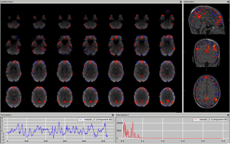
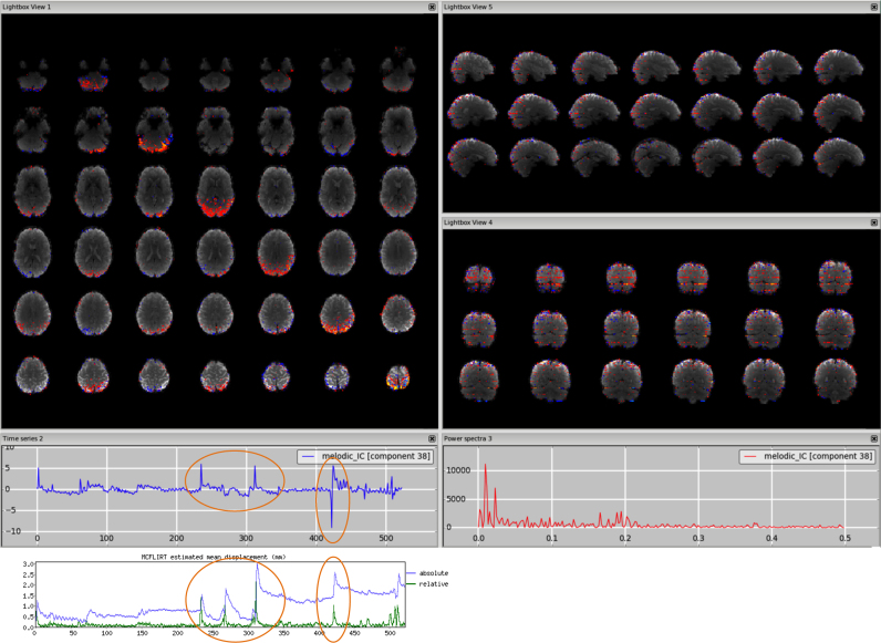
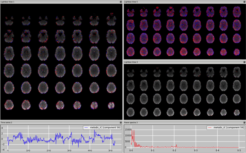
We present a practical "how-to" guide to help determine whether single-subject fMRI independent components (ICs) characterise structured noise or not. Manual identification of signal and noise after ICA decomposition is required for efficient data denoising: to train supervised algorithms, to check the results of unsupervised ones or to manually clean the data. In this paper we describe the main spatial and temporal features of ICs and provide general guidelines on how to evaluate these. Examples of signal and noise components are provided from a wide range of datasets (3T data, including examples from the UK Biobank and the Human Connectome Project, and 7T data), together with practical guidelines for their identification. Finally, we discuss how the data quality, data type and preprocessing can influence the characteristics of the ICs and present examples of particularly challenging datasets.

Fig. 1

Signal. An example signal component showing the Default Mode Network (DMN). The time series (left plot) does not contain sudden jumps and the power spectrum (right plot) is predominantly low frequency. The change of viewing plane and the use of a structural image (e.g. high-resolution T1w) as underlay can help evaluating whether the clusters are localised in the GM (right panel). Threshold z = 2.3.

Fig. 2

Motion artefact. The spatial map presents the typical ring at the edge of the brain and the time series contains a sudden jump in correspondence to sudden head movement, as visible in the motion-correction realignment parameters (highlighted in the orange circles).

Fig. 3

Vein (e.g., sagittal sinus). The vessel is most visible in the sagittal plane, with a structural image as underlay (top-right panel). A similar pattern is visible on smoothed ICA components (in this dataset a smoothing of FWHM = 9.4 mm was applied to the IC maps for visualisation purposes only) (bottom-right panel).

Fig. 4

Arteries. The middle cerebral branches run close to the insula, so a structural image as underlay can help localise the vessels. Changing the threshold (in this case from z = 2.3 to z = 3) helps confirm that the peaks are not in the GM (right panel), although this would probably have been hard to see if the data had been pre-smoothed. This type of component also has a distinctive power spectrum (right plot).

Fig. 5

Cerebrospinal fluid pulsation. The spatial pattern overlaps the third and fourth ventricle, the cisterna magna and the aqueduct of Sylvius (threshold z = 2.3). This is seen most clearly when overlaid onto a structural image looking at a different plane at a higher threshold (top-right panel, z = 3) and after smoothing of the IC map (bottom-right panel).

Fig. 6

Fluctuations in subependymal (and transmedullary) veins. The spatial pattern overlaps the WM-CSF boundary, better localised overlaid onto a structural image (top-right panel). After smoothing of the IC map, the clusters extend more into the WM (bottom-right panel).

Fig. 7

Susceptibility artefacts. Localised on the EPI in areas of signal drop, due mainly to air-tissue interfaces. The use of a higher threshold (in this case from z = 2.3 to z = 4) makes it possible to verify that the peak is in the region of signal drop (right panel).

Fig. 8

Multiband artefact. In the spatial maps, the clusters are visible in a regular way across slices (‘checkerboard’ effects), in this case every 8 (64 slices in z direction, multi band factor 8). This is reflected in stripes in the sagittal and coronal plane (right panels). The spikes in the time series suggest an interaction with head motion (as visible in the motion-correction realignment parameters, highlighted in the orange circles).

Fig. 9

MRI-related artefact. The spatial pattern alternates between positive and negative values (highlighted in the circles on the right panel), and the high frequency spectrum (right plot) and the time series (left plot) are not physiologically meaningful.

Fig. 10

Unclassified noise. In this example, this component has a low frequency spectrum, with a not very smooth time series, a few temporal jumps/discontinuities, and a very scattered spatial pattern. Neither decreasing the threshold (in this case from z = 2.3 to z = 1, top-right panel) or increasing it (in this case from z = 2.3 to z = 4, bottom-right panel) shows any GM cluster that would likely have neural origin.

Fig. 11

Unknown. In this example, the component contains clearly some neural-related signal (DMN), but also some artefacts, possibly of vascular origin, especially visible in the sagittal plane (right panels). The time series is mostly low frequency, but with a high frequency peak as well.

Fig. 12

Unknown. Unlike the former example, there is no clear presence of signal and noise. The spatial pattern is mainly localised in the GM, but is not clearly attributable to an RSN, there is a positive/negative pattern but only on unsmoothed maps, and the power spectrum contains both low and high frequency peaks. Especially in these cases, careful inspection of different planes and smoothed data, also with the underlay of structural image (right panels), is good practice to help determine that the component does not belong to other categories.

Fig. 13

“Innocent until proven guilty” flowchart. A summary of the procedure for visual inspection and manual classification of ICs proposed in this paper. The key points are, first, the importance of evaluating all three pieces of information derived from ICA decomposition (spatial maps, time series and power spectra), although with some hierarchy. Second, the aim of retaining as much signal as possible, and not removing components not clearly identifiable as artefactual. The flowchart does not include natural loops involving double-checking decisions and specific cases, discussed more broadly in the main text.

References

1. Allen E.A., Erhardt E.B., Damaraju E., Gruner W., Segall J.M., Silva R.F., Havlicek M., Rachakonda S., Fries J., Kalyanam R., Michael A.M., Caprihan A., Turner J.A., Eichele T., Adelsheim S., Bryan A.D., Bustillo J., Clark V.P., Feldstein Ewing S.W., Filbey F., Ford C.C., Hutchison K., Jung R.E., Kiehl K.A., Kodituwakku P., Komesu Y.M., Mayer A.R., Pearlson G.D., Phillips J.P., Sadek J.R., Stevens M., Teuscher U., Thoma R.J., Calhoun V.D. A baseline for the multivariate comparison of resting-state networks. Front. Syst. Neurosci. 2011;5:2. - PMC - PubMed
1. Beall E.B., Lowe M.J. Isolating physiologic noise sources with independently determined spatial measures. Neuroimage. 2007;37:1286–1300. - PubMed
1. Beckmann C.F. Modelling with independent components. Neuroimage. 2012;62:891–901. - PubMed
1. Beckmann C.F., DeLuca M., Devlin J.T., Smith S.M. Investigations into resting-state connectivity using independent component analysis. Philos. Trans. R. Soc. Lond. B Biol. Sci. 2005;360:1001–1013. - PMC - PubMed
1. Beckmann C.F., Smith S.M. Probabilistic independent component analysis for functional magnetic resonance imaging. IEEE Trans. Med. Imaging. 2004;23:137–152. - PubMed
Publication types
LinkOut - more resources