Quantitative Frequency-Domain Passive Cavitation Imaging

Abstract

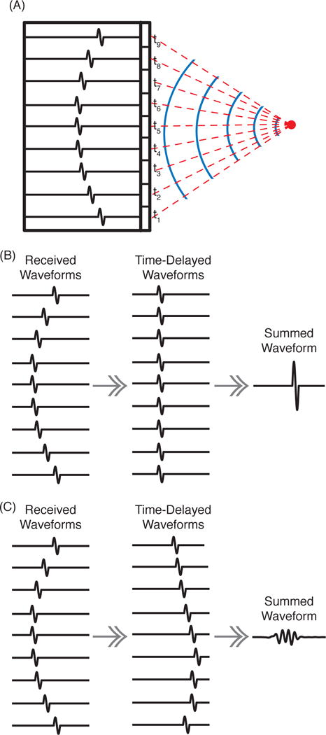
Passive cavitation detection has been an instrumental technique for measuring cavitation dynamics, elucidating concomitant bioeffects, and guiding ultrasound therapies. Recently, techniques have been developed to create images of cavitation activity to provide investigators with a more complete set of information. These techniques use arrays to record and subsequently beamform received cavitation emissions, rather than processing emissions received on a single-element transducer. In this paper, the methods for performing frequency-domain delay, sum, and integrate passive imaging are outlined. The method can be applied to any passively acquired acoustic scattering or emissions, including cavitation emissions. To compare data across different systems, techniques for normalizing Fourier transformed data and converting the data to the acoustic energy received by the array are described. A discussion of hardware requirements and alternative imaging approaches is additionally outlined. Examples are provided in MATLAB.

Fig. 1

(A) An acoustic pulse is emitted from a point source (red circle). The solid blue lines represent wavefronts. The red dashed lines indicate the acoustic propagation paths, each with a corresponding time of flight, t_i. The black outlined rectangles schematically represent the array elements. The recorded waveforms for each element are shown as a single-cycle pulse arriving at different times. (B) When $\overrightarrow{r}$ corresponds to the source location and is used to compute the time delays to shift the waveforms, the waveforms will sum constructively. (C) When $\overrightarrow{r}$ is a location away from the source, the time-delayed waveforms do not add constructively and the summed waveform has a lower amplitude and less energy.

Fig. 2

Example duplex images showing a passive cavitation image (hot colormap) superimposed onto a B-mode ultrasound image using a Philips P4-1 phased array. The cyan box delineates the region of interest over which the passive cavitation image was formed. The passive cavitation images were formed by summing over multiple frequency bands corresponding to (A) ultraharmonic frequencies relative to the insonation frequency (2.23 MHz to 2.27 MHz, 2.73 MHz to 2.77 MHz, and 3.23 MHz to 3.27 MHz) and (B) inharmonic frequencies relative to the insonation frequency (2.105 MHz to 2.145 MHz, 2.605 MHz to 2.645 MHz, and 3.105 MHz to 3.145 MHz). Each passive cavitation image has 15 dB of dynamic range with 0 dB corresponding to the maximum pixel value in each image. (C) Representative energy spectra used to form the passive cavitation images at two different locations, denoted by the green and blue circles in panels A and B, respectively. Note the spatial variation of ultraharmonic and inharmonic components. All of the plots are derived from the same data set.

Fig. 3

An example recorded signal is shown. The signal includes times when only electronic noise was measured by the system (yellow shading), when zero padding as a post-processing step was implemented (orange shading), and when cavitation emissions were recorded (green shading). Only the green shaded region would be including when determining T_IOI.

Fig. 4

Microbubbles were insonified with a 2 MHz pulse of duration 14.4 μs at one of four different pressure amplitudes. The computed energy spectra at the location of the pixel with the maximum amplitude in passive cavitation images is shown (A, B). The energy spectra are plotted on a decibel scale relative to the energy at 4 MHz for each insonation pressure amplitude (A) or relative to the energy at 4 MHz for the 760 kPa insonation (B). Passive cavitation images were formed for each insonation pressure amplitude from the energy at the ultraharmonic frequency of 7 MHz, shown with green shading [(C), (D), (E), (F), respectively] and the inharmonic frequency of 4.5 MHz shown with red-orange shading [(G), (H), (I), (J), respectively]. For comparison, subfigures (K), (L), (M), and (N) are formed using a time-domain algorithm, which beamforms all frequencies. For a given bandwidth, each image was normalized by the maximum energy in the image formed from data obtained while insonifying with a 760 kPa peak rarefactional pressure amplitude.

Fig. 5

Schematics of possible alignment strategies between the imaging array (gray) and insonation transducer (white). The perimeter of the focal volume of the insonation transducer is denoted by the red line. The point-spread-function of the imaging array is shown as yellow shading. Jensen et al., [34] used a coaxial alignment, which relies on a single acoustic window (or path) through the body. However, the point-spread-function of the imaging array overlaps entirely with the focus of the insonation transducer, preventing resolution of cavitation activity at different locations within the focal volume. Perpendicular alignments have enabled the resolution of cavitation activity within the focus, but require separate acoustic paths to enable colocation of the foci [37], [43]. The acute alignment, such as the experimental setup used by Choi et al., [45] provides another option for co-alignment to resolve cavitation activity within the insonation transducer focal volume.

References

1. Mellen RH. Ultrasonic Spectrum of Cavitation Noise in Water. J Acoust Soc Am. 1954 May;26(3):356–360.
1. Kremkau FW, Gramiak R, Carstensen EL, Shah PM, Kramer DH. Ultrasonic detection of cavitation at catheter tips. Am J Roentgenol Radium Ther Nucl Med. 1970 Sep;110(1):177–183. - PubMed
1. Atchley AA, Frizzell LA, Apfel RE, Holland CK, Madanshetty SI, Roy RA. Thresholds for cavitation produced in water by pulsed ultrasound. Ultrasonics. 1988;26:280–285. - PubMed
1. King DA, O’Brien WD. Comparison bewteen maximum radial expansion of ultrasound contrast agents and experimental postexcitation signal results. J Acoust Soc Am. 2011;129(1):114–121. - PMC - PubMed
1. Radhakrishnan K, Bader KB, Haworth KJ, Kopechek JA, Raymond JL, Huang S-L, McPherson DD, Holland CK. Relationship between cavitation and loss of echogenicity from ultrasound contrast agents. Phys Med Biol. 2013;58(18):6541–6563. - PMC - PubMed
Publication types