Automated Multi-Peak Tracking Kymography (AMTraK): A Tool to Quantify Sub-Cellular Dynamics with Sub-Pixel Accuracy

Abstract

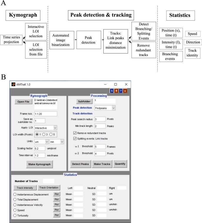
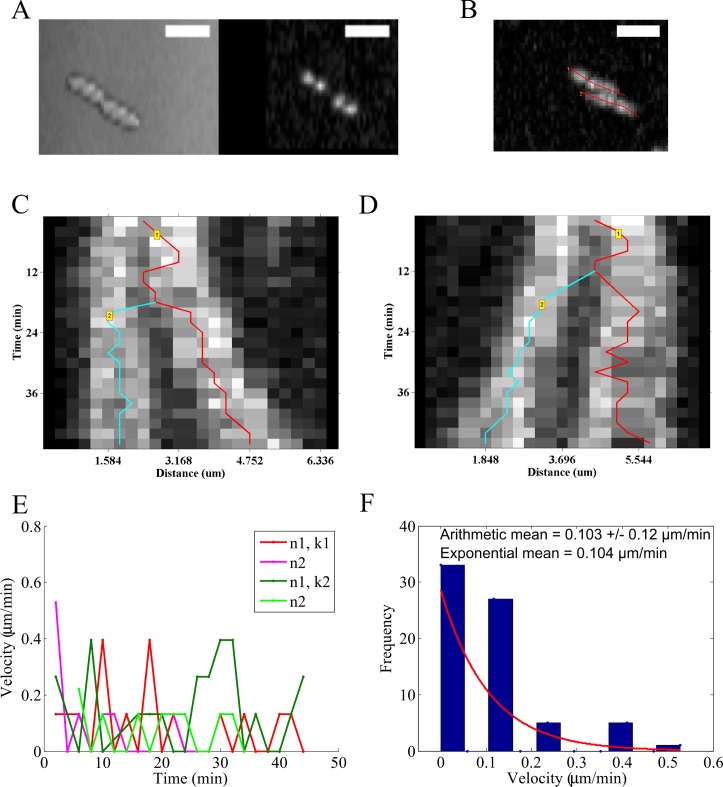
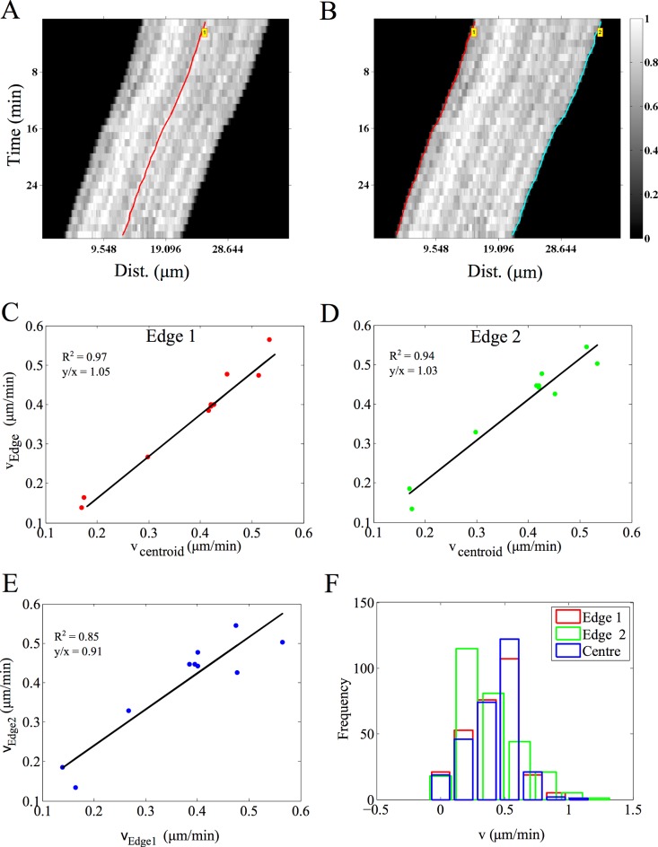
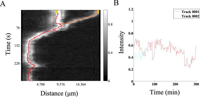
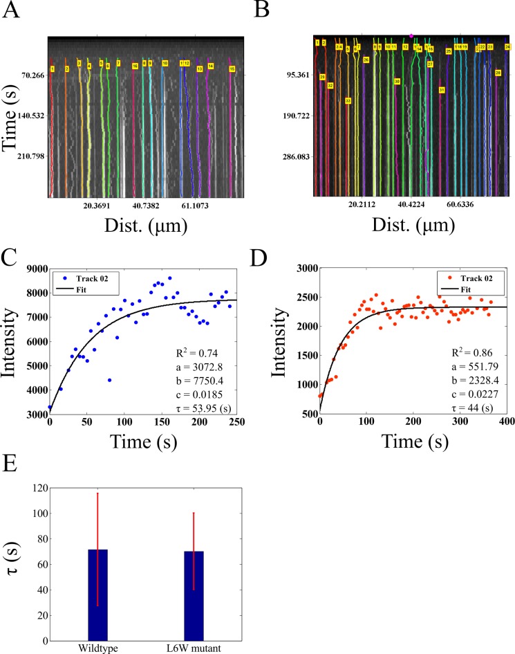
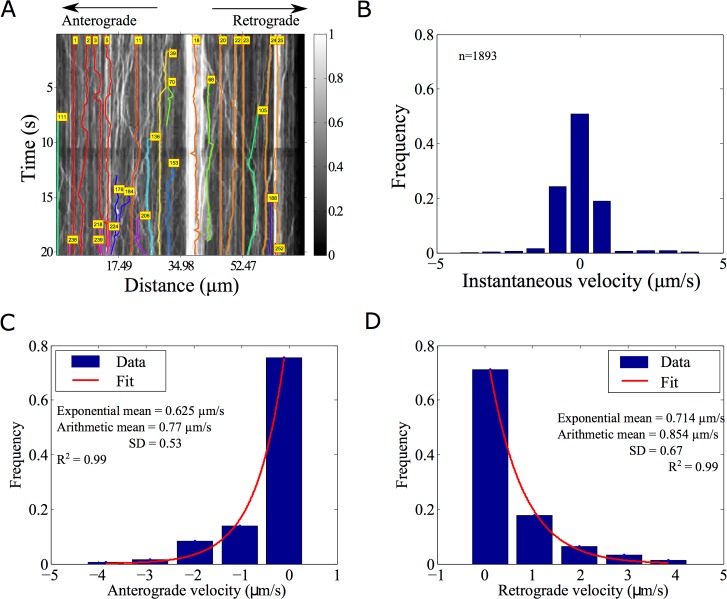
Kymographs or space-time plots are widely used in cell biology to reduce the dimensions of a time-series in microscopy for both qualitative and quantitative insight into spatio-temporal dynamics. While multiple tools for image kymography have been described before, quantification remains largely manual. Here, we describe a novel software tool for automated multi-peak tracking kymography (AMTraK), which uses peak information and distance minimization to track and automatically quantify kymographs, integrated in a GUI. The program takes fluorescence time-series data as an input and tracks contours in the kymographs based on intensity and gradient peaks. By integrating a branch-point detection method, it can be used to identify merging and splitting events of tracks, important in separation and coalescence events. In tests with synthetic images, we demonstrate sub-pixel positional accuracy of the program. We test the program by quantifying sub-cellular dynamics in rod-shaped bacteria, microtubule (MT) transport and vesicle dynamics. A time-series of E. coli cell division with labeled nucleoid DNA is used to identify the time-point and rate at which the nucleoid segregates. The mean velocity of microtubule (MT) gliding motility due to a recombinant kinesin motor is estimated as 0.5 μm/s, in agreement with published values, and comparable to estimates using software for nanometer precision filament-tracking. We proceed to employ AMTraK to analyze previously published time-series microscopy data where kymographs had been manually quantified: clathrin polymerization kinetics during vesicle formation and anterograde and retrograde transport in axons. AMTraK analysis not only reproduces the reported parameters, it also provides an objective and automated method for reproducible analysis of kymographs from in vitro and in vivo fluorescence microscopy time-series of sub-cellular dynamics.

Fig 1. Algorithm workflow and user-interface.

(A) The workflow of the algorithm involves three steps (1) kymograph generation, (2) peak detection and tracking and (3) quantification and the functions invoked by each part are elaborated. (B) The GUI is organized to reflect this workflow.

Fig 2. Estimating positional accuracy.

(A) A single frame of a 2D image time-series of static spheres (with a peak intensity of 1) with Gaussian noise (mean = 0, s.d. = 40) is analyzed using AMTraK (B) resulting in a kymograph. (C) The frequency distribution of the error in position detection (Δx) by AMTraK (bars) is fit by an exponential decay (red). The mean error obtained is 0.75 pixels (goodness of fit R² = 0.95) for a representative time-series with noise s.d. = 40. (D) The mean error of detection (y-axis) from the exponential fit <Δx> = 1/b (black) is compared to the arithmetic mean (blue) in pixel units, plotted as a function of increasing noise s.d. (x-axis). The noise generates random intensities drawn from a Gaussian distribution with mean 0 and the specified s.d. being added to the image (based on the “Specified Noise” function in ImageJ).

Fig 3. Positional accuracy of tracking simulated motility.

(A) Kymographs of time-series of spheres undergoing a 1D random walk with Gaussian noise (s.d. = 30) were tracked. The colors indicate the detected tracks. (B) The arithmetic mean (blue) and exponential mean (black) of error in position detection (Δx) (y-axis) over 3 iterations of the time-series is plotted for increasing velocity of the random-walk (x-axis) as inferred from the standard deviation (s.d.).

Fig 4. Nucleoid segregation dynamics of E. coli.

(A) Image time-series of E. coli MG1655 grown on agar pads and imaged in DIC (left) and fluorescence based on HupA-GFP (right) are analyzed using AMTraK. (B) AMTraK generates a maximum intensity projection on the basis of which user-selected lines of interest (red lines) are used by the program to generate kymographs. The kymographs based on (C) LOI 1 (k1) and (D) LOI 2 (k2) were tracked resulting in branched tracks (colored lines). (E) The instantaneous velocities of nucleoids 1 and 2 (n1, n2) from kymographs 1 (k1) and 2 (k2) are plotted as a function of time (colors indicate nucleoids n1, n2 each from the kymographs k1, k2). (F) Mean velocities are estimated using both the arithmetic mean (±s.d.) and v_ex, the mean of the exponential decay (y = e^-1/vex) that was fit (red line) to the frequency distribution of instantaneous velocity (bars). Scale bar 4 μm.

Fig 5. Microtubule (MT) gliding motility on kinesin motors.

MTs gliding on kinesin (images acquired every 1 minute for 30 minutes) were analyzed using AMTraK by either detecting (A) the centerline (red) or (B) the two edges the filament, edge 1 (red) and 2 (cyan). Color bar: gray scale image intensity normalized by the maximal value for the bit-depth. (C, D) The velocity estimates from the centroid-based velocity estimates and the two edges and (E) the velocity estimated from each edge are correlated. (F) The frequency distribution of the instantaneous velocity estimates using the centroid (blue) is compared to edge-based estimates. r²: goodness of fit, y/x: slope of the linear fit. Number of filaments analyzed, n = 10.

Fig 6. MT aster coalescence.

(A) A time-series of MT asters undergoing fusion (time-series taken from previous work by Foster et al. [39]) was analyzed using AMTraK. The grey scale bar indicates normalized fluorescence intensity of Alexa-647 labeled tubulin. (B) The relative intensity over time of the two coalescing asters is plotted.

Fig 7. Dynamics of clathrin assembly.

(A, B) Microscopy time-series taken from Holkar et al. [24] of fluorescently labeled clathrin assembly in the presence of (A) wild-type and (B) mutant epsin were analyzed using AMTraK. Colored lines in the kymographs indicate detected tracks. (C, D) The change in intensity as a function of time based on AMTraK detected tracks from (C) clathrin + w.t. epsin and (D) compared to clathrin + (L6W) mutant epsin. The intensity kinetics plots are fit to a single-phase exponential function, y = a+(b-a)*(1-e^-c*t) to obtain the time constant of assembly τ = 1/c (red). R²: goodness of fit. (D) The mean values (error bar represents s.d.) of the time constant of assembly of clathrin (τ) in the presence of wild-type and mutant epsin are compared.

Fig 8. Analysis of synaptic vesicle transport.

(A) GFP-Rab3 tagged vesicles from posterior touch cell neurons in C. elegans (experimental data from taken from supporting movie S1 Movie from [28]) were analyzed using AMTraK. Colored lines with index numbers indicate tracks. (B) The frequency distribution of instantaneous velocities of the vesicles (n = 1592) is plotted using AMTraK (mean: 0.49 μm/s, s.d. 0.88). (C, D) The frequency distribution of non-zero velocities are fit with an exponential decay function y = A*e^-x/m (red line), where A: scaling factor and m: mean. (C) The mean anterograde velocity from the fit is 0.625 μm/s with arithmetic mean 0.77±0.53 μm/s (n = 425) and (D) the mean retrograde velocity from the fit is 0.714 μm/s with arithmetic mean 0.854±0.67 μm/s (n = 540). Arithmetic means are reported ± standard deviation (s.d.). R² indicates the goodness of the fit.

References

1. Pereira AJ, Maiato H (2010) Improved kymography tools and its applications to mitosis. Methods 51: 214–219. 10.1016/j.ymeth.2010.01.016 - DOI - PubMed
1. Rietdorf J, Seitz A (2008) Multi Kymograph. Available: http://fiji.sc/Multi_Kymograph.
1. Chetta J, Shah SB (2011) A novel algorithm to generate kymographs from dynamic axons for the quantitative analysis of axonal transport. J Neurosci Methods 199: 230–240. Available: http://www.ncbi.nlm.nih.gov/pubmed/21620890. 10.1016/j.jneumeth.2011.05.013 - DOI - PubMed
1. Chiba K, Shimada Y, Kinjo M, Suzuki T, Uchida S (2014) Simple and direct assembly of kymographs from movies using KYMOMAKER. Traffic 15: 1–11. 10.1111/tra.12127 - DOI - PubMed
1. Chenouard N, Buisson J, Bloch I, Bastin P, Olivo-Marin J-C (2010) Curvelet analysis of kymograph for tracking bi-directional particles in fluorescence microscopy images. IEEE International Conference on Image Processing (ICIP). http://icy.bioimageanalysis.org/plugin/KymographTracker.