Inferring human microbial dynamics from temporal metagenomics data: Pitfalls and lessons

Abstract

The human gut microbiota is a very complex and dynamic ecosystem that plays a crucial role in health and well-being. Inferring microbial community structure and dynamics directly from time-resolved metagenomics data is key to understanding the community ecology and predicting its temporal behavior. Many methods have been proposed to perform the inference. Yet, as we point out in this review, there are several pitfalls along the way. Indeed, the uninformative temporal measurements and the compositional nature of the relative abundance data raise serious challenges in inference. Moreover, the inference results can be largely distorted when only focusing on highly abundant species by ignoring or grouping low-abundance species. Finally, the implicit assumptions in various regularization methods may not reflect reality. Those issues have to be seriously considered in ecological modeling of human gut microbiota.

Keywords: dynamics inference; ecological modeling; human microbiome; temporal metagenomics.

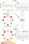
Figure 1.

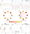
Overview of the workflow inferring microbial dynamics from time-series data. Given suitable perturbations (A) on a microbial ecosystem, and the corresponding time-series of microbe abundances (B), we aim to infer the microbial dynamics and reconstruct the underlying microbe-microbe interaction network (C) by using classical population dynamics models, e.g. the Generalized Lotka-Volterra (GLV) model, and various standard system identification techniques (D). In the ideal case, the reconstructed microbe-microbe interaction network (E) captures all the key features of the original network (C), and the predicted time-series (F) agrees well with the original measurement (B). Yet, as pointed in this paper, there are many pitfalls in inferring the microbial dynamics from time-series data. In both (C) and (E), positive (or negative) interactions are shown in blue (or red) arrows, respectively. The absolute interaction strengths are proportional to the arrow widths and the microbiota growth rates are represented by circle colors. NRMSE represents the normalized root mean square error.

Figure 2.

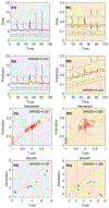
Perfect time-series prediction does not imply accurate network reconstruction. A1: Time-series of binary perturbations. A2: Synthetic time-series of species abundances generated from a GLV model. Both perturbation and abundance data are sampled once per day. A3: Predicted time-series of species abundances calculated from the inferred GLV model. B1: Original inter-species interaction network. B2: Reconstructed inter-species interaction network. Here in both B1 and B2 only the top-10 strongest interactions are shown. Circle colors represent growth rates. C1: Inferred interaction strengths versus true interaction strengths. C2: Inferred growth rates versus true growth rates. C3: Inferred susceptibilities versus true susceptibilities.

Figure 3.

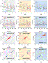
Impact of sampling rates on inferring microbial dynamics. Row-1: Time-series of species abundances generated from a GLV model with different sampling rates: (A1): once a week; (B1): every two days; (C1): daily; and (D1): twice a day. Row-2: Predicted time-series of species abundances calculated from the corresponding inferred GLV model. Row-3: True interaction strengths versus inferred interaction strengths from time-series data of different sampling rates. Row-4: True growth rates versus inferred growth rates from time-series data of different sampling rates.

Figure 4.

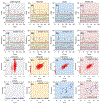
Compositionality of relative abundance data impedes the inference of microbial dynamics. Column-1: using absolute abundance data. A1: Time-series of absolute abundances; A2: Predicted time-series of absolute abundances; A3: True interaction strengths versus inferred interaction strengths; A4: True growth rates versus inferred growth rates. Column-2: using relative abundance data. B1 Time-series of relative abundances; B2: Predicted time-series of relative abundances; B3: True interaction strengths versus inferred interaction strengths; B4: True growth rates versus inferred growth rates. Inference results from relative abundances are far from the ground truth. The time-series prediction of relative abundances also differs significantly from that of the original relative abundances.

Figure 5.

Ignoring or grouping low-abundance species impedes the inference of microbial dynamics. Column A: Without ignoring or grouping of low-abundance species, the inference results are acceptable, and the predicted time-series agrees well with the original time-series data, provided the sampling rate is high enough. Column B: After ignoring the low-abundance species, the inference results are much worse, despite the predicted time-series still agrees well with the original time-series data. Column C: If we group the low-abundance species together and regard them as a new species, the inference results are still not comparable to the results of using original data. In generating these figures, we consider a system of n = 15 species with a heterogeneous inter-species interaction network with mean degree <k> = 11.2.

Figure 6.

Inappropriate regularization impedes the inference of microbial dynamics. Column A: Without any regularization, we can perform the inference using the least-square method (i.e. no penalty terms). The inference results are not acceptable. Column B: With Tikhonov regularization (also known as ℓ²-regularization or ridge regression), the inference results are still bad. Column C: With lasso regularization (also known as ℓ¹-regularization), the inference results are slightly better. Column D: With elastic net regularization, which uses a linear combination of ℓ¹- and ℓ²-norm penalty terms (with μ = 0:5 in equation (10)), the inference results are as good as that of using lasso only. Note that in all the four cases, the predicted time-series agrees well with the original time-series data. In generating these figures, we consider a microbial ecosystem of n = 30 species with a homogeneous inter-species interaction network and mean degree 〈k〉 = 23:2.

References

1. Sender R, Fuchs S, Milo R. 2016. Revised estimates for the number of human and bacteria cells in the body. PLoS Biol 14: 1–14. - PMC - PubMed
1. Clemente JC, Ursell LK, Parfrey LW, Knight R. 2012. The impact of the gut microbiota on human health: an integrative view. Cell 148: 1258–70. - PMC - PubMed
1. Consortium H. 2012. Structure, function and diversity of the healthy human microbiome. Nature 486: 207–14. - PMC - PubMed
1. Consortium H. 2012. A framework for human microbiome research. Nature 486: 215–21. - PMC - PubMed
1. Costello EK, Stagaman K, Dethlefsen L, Bohannan BJM, et al. 2012. The application of ecological theory toward an understanding of the human microbiome. Science 336: 1255–62. - PMC - PubMed
Publication types
LinkOut - more resources