Magnification calibration and the determination of spherical virus diameters using cryo-microscopy

Abstract

The diameters of several frozen-hydrated, spherical viruses were determined using polyoma virus as either an external or an internal calibration standard. The methods described provide a reproducible and accurate way to calibrate microscope magnification. The measured diameters are in excellent agreement with respective measurements previously reported for aqueous samples at room temperature using X-ray diffraction methods. These results indicate that the native morphology and dimensions of biological macromolecules are better preserved in frozen-hydrated samples when compared with more conventional electron microscopy techniques such as negative-staining, metal shadowing or thin-sectioning.

Fig. 1

Determination of virion image radius. (A) Digital image of an unfiltered, floated, circularly boxed polyoma virion. The virion image is displayed with enhanced positive contrast. The higher density of the virus compared to the surrounding vitrified water makes it appear darker. The center and edge of the particle are identified respectively by the base and tip of the arrow (same for B). (B) Image shown in (A) circularly averaged about the particle center. The particle edge is easier to identify compared to (A) due to the abrupt change in the averaged density. (C) Radial density plot corresponding to the intensities along the arrow in (B). The arrow identifies the location of the particle boundary. Since the position of the abscissa axis is established by the floating procedure, there is some uncertainty in identifying the exact position of the particle boundary, although the uncertainty is small since the abrupt change in contrast is confined to a narrow range of radii.

Fig. 2

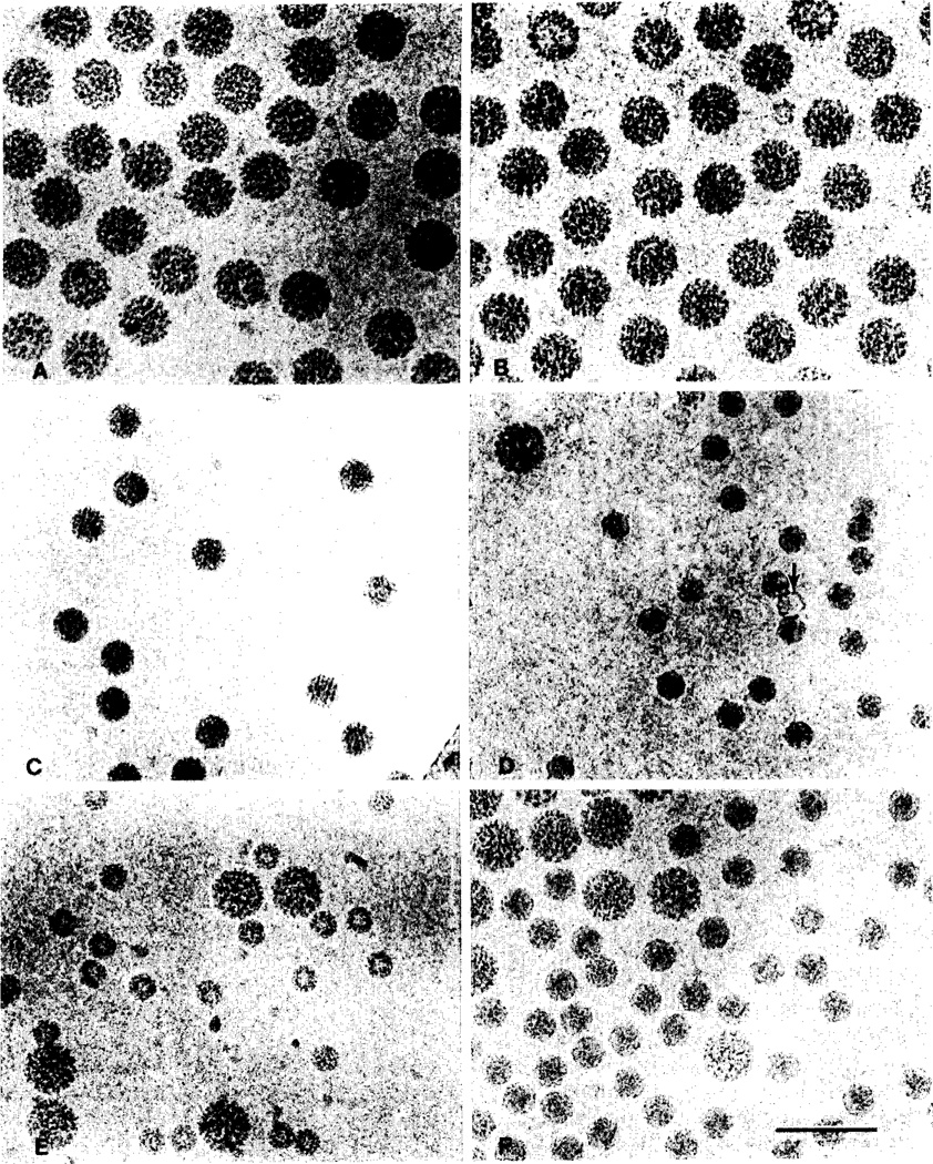
Unstained, frozen-hydrated spherical viruses, suspended over holes in a carbon substrate. Magnification is identical for all images (bar = 100 nm). (A) Polyoma. (B) SV40. (C) NβV. (D) CPMV/polyoma mixture; the arrow identifies a CPMV empty capsid. (E) BMV/polyoma mixture. (F) FHV/polyoma mixture.

Fig. 3

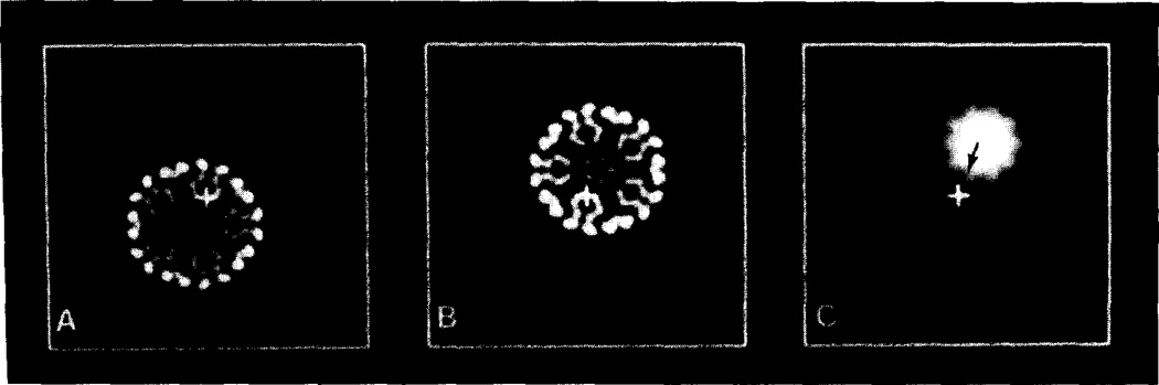
Cross-correlation method for initial location of the center of images of “spherical” particles. (A) Incorrectly “boxed” image of a model T = 3 icosahedral particle, viewed down a five-fold axis. The center of the model is slightly below and to the left of the box center (“ + ”). (B) Same as (A) after 180° rotation. (C) Cross-correlation pattern between (A) and (B). The vector difference between the highest peak in the cross-correlation pattern (base of arrow) and the origin of the pattern (“ + ”), identifies the direction and magnitude of the difference between the centers of the unrotated (A) and rotated (B) model images. The center of the particle in (A) is one-half the vector distance identified in (C) from the center of the “boxed” area in (A).

Fig. 4

Pattern produced by cross-correlating a polyoma virion image with the same image rotated by 180°. The inset at the upper right is a magnified contour display of the center of the pattern. This facilitates the location of the peak position in the cross-correlation pattern using an interactive graphics cursor (“×”).

Fig. 5

Cross-correlation procedure to select and average virion images. (A) Image of a frozen-hydrated mixture of polyoma (larger particles) and FHV. The increase in average background density from left to right is due to an increase in vitrified water thickness over the hole in the carbon substrate. (B) Fourier-space “ prefiltered” image of (A) obtained by Fourier reconstruction methods [66] which remove low frequency fluctuations ( > ~ 100 nm) mainly contributed by the variation in the thickness of the vitrified water. The circled FHV (left) and the polyoma (right) images were used a reference images for the cross-correlation procedure. Both reference particles were boxed with identical size circular boundaries to minimize ambiguities in discriminating correlation peaks for the two different virions (see footnote in appendix B). (C) Schematic representation of (B), identifying the approximate location of the FHV and polyoma particles. (D) Cross-correlation pattern between the polyoma reference (circled in (B)) and image (A). Areas of high correlation are represented by brighter colors. The arrow identifies the strongest correlation peak, locating the polyoma reference. (E) Cross-correlation pattern between the polyoma reference circled in (B)) with image (B). The removal of low-frequency features enhances the ability to clearly identify all the polyoma positions. Virion images in (B), identified by the peaks, were averaged, and this average was used as the reference in a subsequent cycle of cross-correlation averaging. (F) Cross-correlation pattern between the reference average image and (B). The peaks identifying the positions of the polyoma particles are much sharper and clearer than those in (E). The inset shows the averaged polyoma image obtained by combining those particles identified by the peaks in the last correlation pattern computed. (G) Same as (D) with the exception that the FHV image circled in (B) was used as the reference. The arrow locates the position of the FHV reference. (H) Same as (E) using the FHV reference (circled in (B)). (I) Same as (F) using an averaged FHV image. The inset shows the averaged FHV image obtained after the second cycle of correlation averaging.