Measurement of amyloid formation by turbidity assay-seeing through the cloud

Abstract

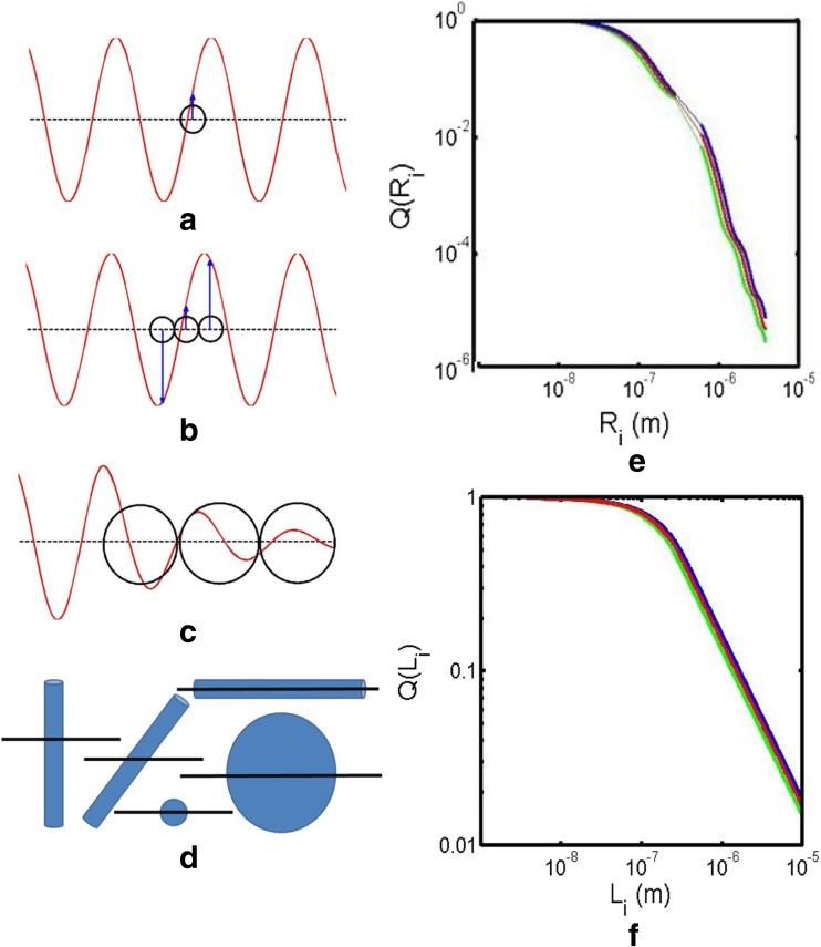
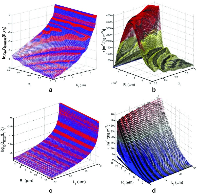
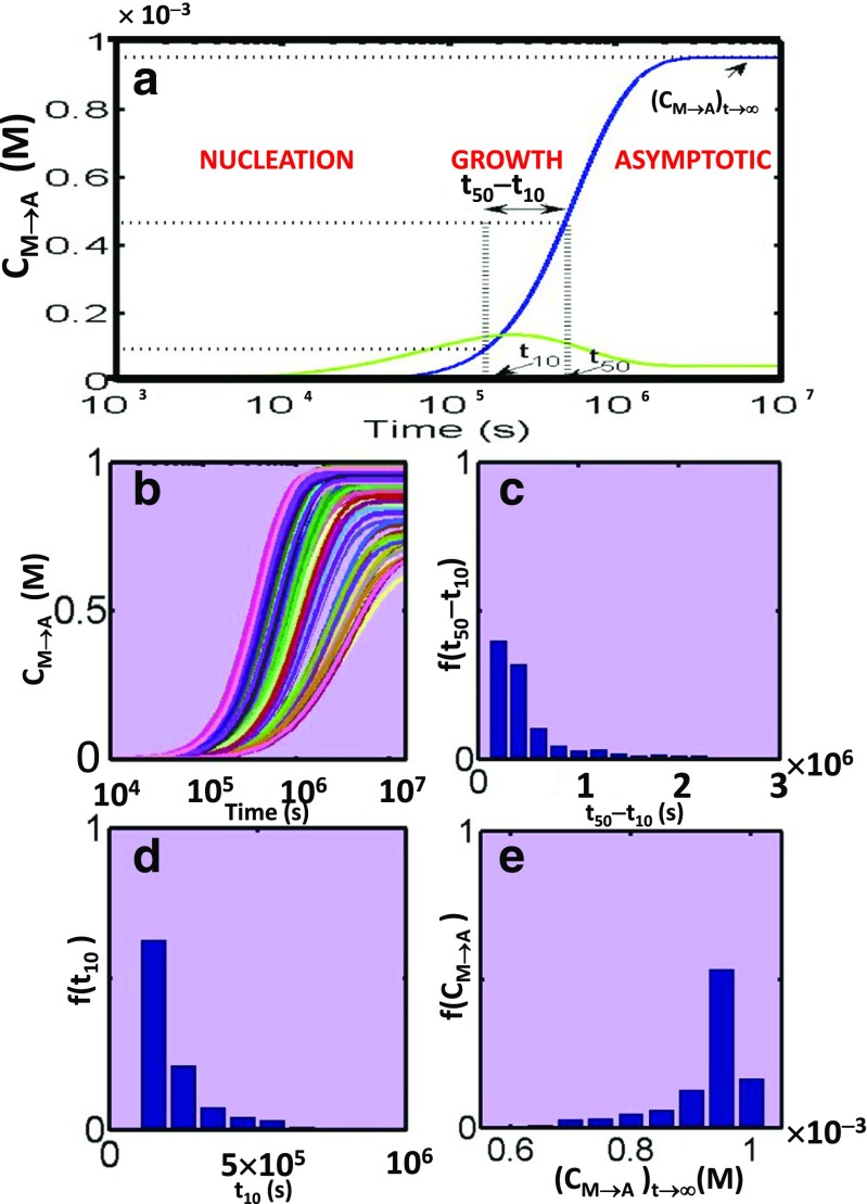
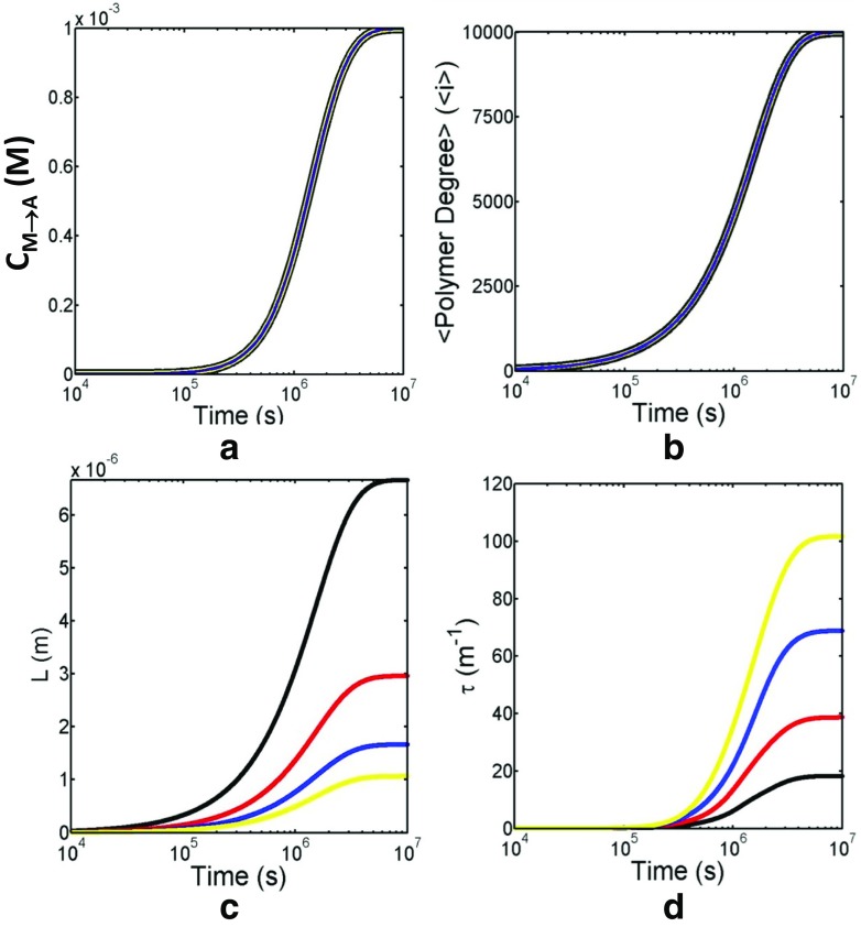
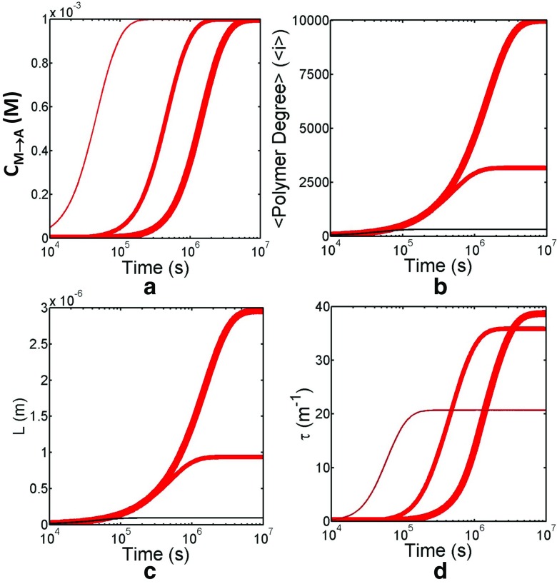
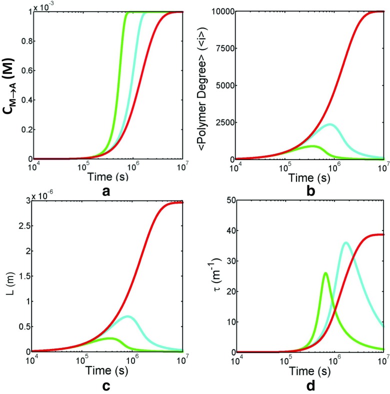
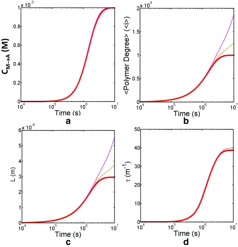
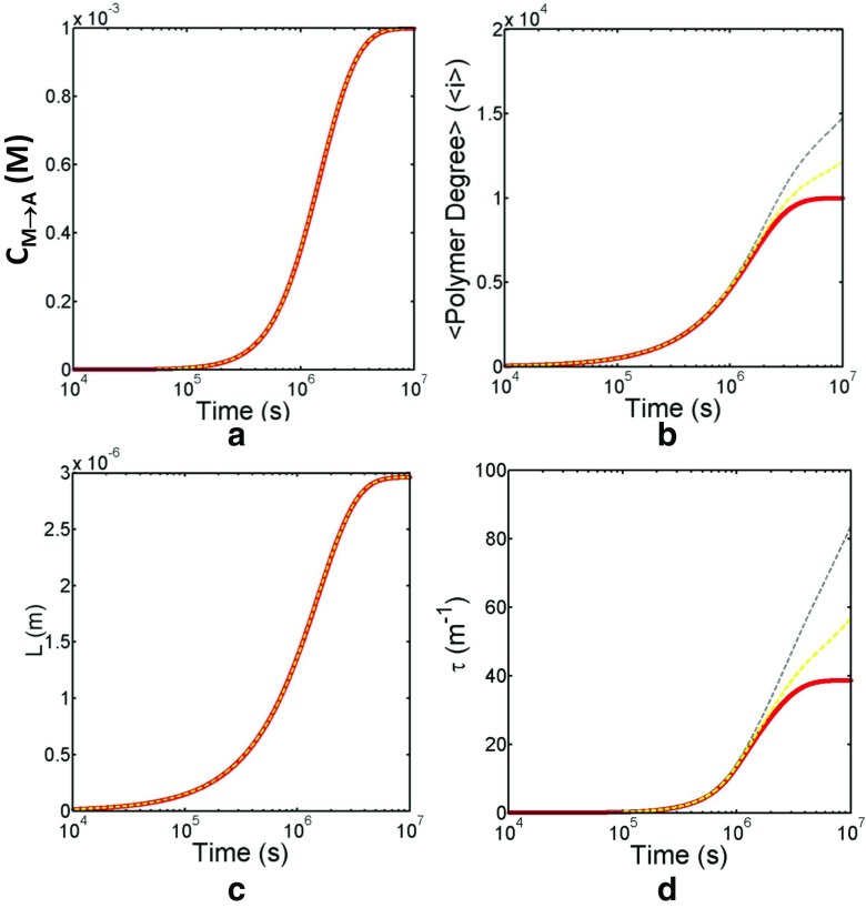
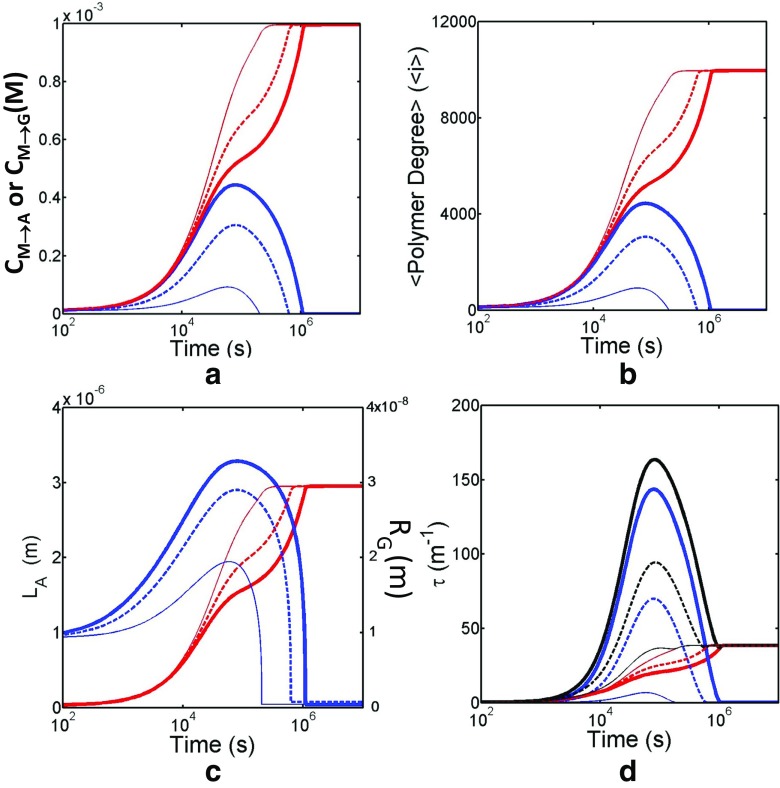
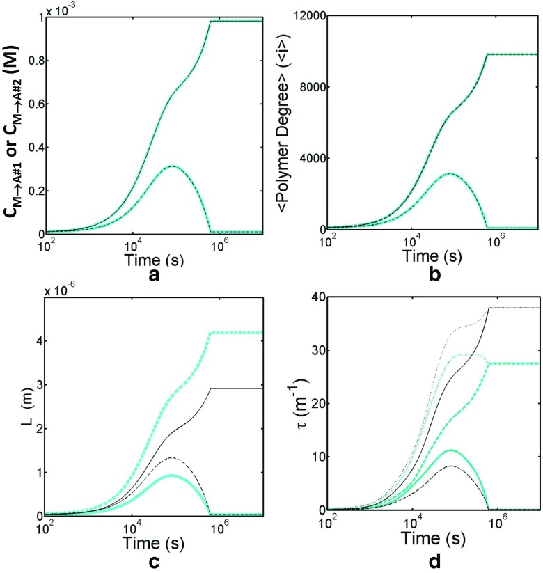
Detection of amyloid growth is commonly carried out by measurement of solution turbidity, a low-cost assay procedure based on the intrinsic light scattering properties of the protein aggregate. Here, we review the biophysical chemistry associated with the turbidimetric assay methodology, exploring the reviewed literature using a series of pedagogical kinetic simulations. In turn, these simulations are used to interrogate the literature concerned with in vitro drug screening and the assessment of amyloid aggregation mechanisms.

Keywords: Amyloid aggregation kinetics; Amyloid biophysics; Data reduction; Nonlinear signal response; Turbidimetric method.

Fig. 1

Amyloid structure. a Consensus structural features of the amyloid fibre. Left Intermolecular β-sheet stacks are formed between polypeptides along the direction of the fibre. One or more sections of a polypeptide may contribute to the longitudinal β-sheet formation. Hydrophobic-driven lateral packing may occur between the orthogonal faces of the β-sheet elements within the amyloid fibre. Centre The simplest possible fibre arrangement is termed a protofibril which can be characterized by a length, width, persistence length and helical pitch. Right Hydrophobic packing forces can cause multiple protofibrils to align to yield higher-order quaternary arrangements of amyloid fibres termed ‘mature fibres’ (figures adapted, with permission, from Hall and Edskes 2012). b Artistic renderings of the structures of four different amyloids solved by a combination of solid-state nuclear magnetic resonance and various types of electron microscopy. From left to right amyloid fibres derived from the human prion protein (Apostol et al. 2010), yeast prion amyloid fibres formed from the full-length yeast protein HET-s (Van Melckebeke et al. 2010), amyloid formed from a peptide segment of transthyretin (Fitzpatrick et al. 2013) and a mature amyloid fibre, composed of multiple protofibrils, derived from the brain of an Alzheimer’s Disease patient (Paravastu et al. 2008). Bar in lower left hand corner 5 nm [figures adapted from painted illustrations by D.G. Goodsell (Goodsell et al. 2015)]

Fig. 2

Ultramicroscopy-based analysis of protein aggregates can provide the necessary mesoscopic-level structural information for estimating turbidity via the methods outlined in the text of this review. a Typical experimental transmission electron microscopy (TEM) image of amyloid fibres (made from pig insulin at pH 3.0 and 60 °C, recorded at 6000× magnification (adapted, with permission, from Fig. 9 of Hall 2012). b Example of a pseudo-TEM image generated using the Amyloid Distribution Measurement (ADM) software useful for calibrating and testing image analysis routines and designing better ultramicroscope experiments (adapted, with permission, from Fig. 2 of Hall 2012). c Mesoscopic representation of fibre by a sphero-cylinder of variable internal length (L) and width (W) (adapted, with permission, from Fig. 8 of Hall 2012). d Average angle of deviation (θ_av) for an individual fibre as determined by Hall et al. (2016a) using successive calculation of the dot product between projection vectors that trace along the backbone of the amyloid fibre (adapted, with permission, from Fig. 3a of Hall 2012). e Analysis of simulated TEM data yielding two-dimensional histograms of length and width (adapted, with permission, from Fig. 12 of Hall 2012). f Analysis of simulated TEM data yielding two-dimensional histogram of width and average deviation (adapted, with permission, from Fig. 12 of Hall 2012)

Fig. 3

Coarse structural models of aggregates. a Schematic describing coarse-grained conceptualization of bonding arrangements seen in various types of protein aggregate corresponding to amorphous (left), crystalline (middle) and fibrous (right) structures. b Schematic describing mesoscopic structural groupings of aggregates as either rod-like or spherical with assignment of a volume packing fraction, defined by the parameter α, such that a darker colour represents a greater fractional occupancy of the aggregate trace volume by protein, i.e. a greater internal density (schematic is adapted, with permission, from Fig. 1 of Hall et al. 2016a, b)

Fig. 4

Principles of light scattering. a Schematic describing the transmission-based measurement of excess solution turbidity of protein aggregates in which the transmitted light intensity (I _T) is measured in relation to the incident light intensity (I ₀) using a standard spectrophotometer (or plate reader). b Ray diagram of the encounter between light and the scattering particle in solution. c Simplified schematic of a general goniometric scattering experiment for non-polarized light (although the light wave shown has only one polarization!). Scattering intensity for Rayleigh-type scattering is equivalent when recorded at any point on a sphere (centre located at the scattering particle) defined by the radius (r) and the angle θ, whereby θ is defined as the sub-apex of the spherical solid angle measured from the forward scattering direction (adapted, with permission, from Fig. 2a of Hall et al. 2016a, b). d Colour plot indicating the scattering intensity (normalized relative to the scattering recorded at right angles to the incident beam) as a function of the recording angle θ, with the system conforming to limiting Rayleigh scattering conditions described in c (adapted, with permission, from Fig. 2b of Hall et al. 2016a, b)

Fig. 5

Theoretical treatments of scattering. a–c Three general scattering regimes were considered by Hall et al. (2016a), namely a Rayleigh limit—where the scattering particle is small in relation to the wavelength of light [<R_i> < λ/20] (red line light wave, blue arrow position of the dependent electric field vector). b Rayleigh–Gans–Debye limit—where the particle can be reasonably large in relation to the wavelength of light at ∼[0 < <R_i> < λ/2] such that it produces out-of-phase scattering at different centres of the particle but the light suffers no appreciable loss of intensity as it passes through the particle. c Mie scattering regime—where the particle is sufficiently large to both generate out-of-phase scattering and to perturb the intensity of the light as it passes through the aggregate. For the anomalous diffraction approximation of the Mie equation used by Hall et al. (2016a) this description is applicable over the size regime of ∼[2λ < <R_i> < 15λ]. d Schematic highlighting the potential for orientation effects on both the out-of-phase scattering and loss of intensity complications accompanying increasing size and asymmetry of the aggregate. All quantitative descriptions described by Hall et al. (2016a) assume random orientation of the aggregate. e Continuous description of the transmittance form factor for a spherical aggregate [Q(R_SPHERE)] at three different wavelengths (blue line 400 nm, red line 450 nm, green line 500 nm). Interpolation based on a polynomial description of spliced simulations from the three characteristic size regimes is shown in Table 1. f Continuous description of the transmittance form factor for rods [Q(L_ROD)] over a large size regime for three different wavelengths (a–d adapted, with permission, from Fig. 3 of Hall et al. ; e, f adapted, with permission, from Fig. 5 of Hall et al. 2016a)

Fig. 6

Utilitarian approach developed by Hall et al. (2016a, b) for estimating turbidity. a Two-dimensional polynomial fit of simulated Q values for a sphere: fitted values were overlaid onto large sets of the base ten logarithm of Q calculated for a sphere of arbitrary packing fraction α_I and radius R_i, determined using the interpolation technique describe in Fig. 5e (at λ = 400 nm). b Specific turbidity (turbidity per kg/m³ of aggregate) for a spherical protein aggregate of arbitrary α_i and R_i, calculated using the corresponding value of Q shown in a. Protein concentration and mass were respectively set at 1 mg/ml and 5000 g/mole. c, d Corresponding plots to a and b, respectively, but this time describing the case for cylindrical rods of arbitrary length and radius. Specific turbidity in d was calculated at the same concentration and mass of the protein monomer with a value of the specific fractional volume occupancy of α = 1.0 (adapted, with permission, from Figs. 6, 7, 8 and 9 of Hall et al. 2016a, b)

Fig. 7

Schematic of amyloid kinetics. a Characteristic features of amyloid nucleation–growth polymerization kinetics include a characteristic lag/nucleation phase, a steep growth phase and an asymptotic endpoint. A simple scheme for reducing the data to parameters reflecting each of these characteristic features is included. These parameters include (1) the kinetic tenth time, t ₁₀ (time to reach 10 % of reaction), reflecting the nucleation phase, (2) a composite term reflecting the difference between half-time, t ₅₀, and kinetic tenth time (t ₅₀ − t ₁₀) characteristic of the growth phase and (3) the time-independent value of the extent of the monomer incorporated into amyloid, (C _M→A)_t→∞, characterizing the asymptotic phase. Blue line Value of C_M→A as a function of time, green line the corresponding concentration of monomer as critical nucleus (nC_N) as a function of time (adapted, with permission, from Fig. 1d of Hall et al. 2016a, b). b Data reduction and analysis. In the case of drug screening for amyloid inhibitors, replicate measurements of the measured growth kinetics are decomposed into a set of characteristic values (such as the set of parameters described in Fig. 7a), with resultant values represented as a fractional histogram. c–e Fractional histogram representation of the surrogate markers of the nucleation (d), growth (c) and asymptotic (e) regions derived from the simulations shown in b (adapted, with permission from Fig. 2 of Hall et al. 2016b), with simulated results multiplied by a constant value to more closely reflect the time course and concentration profiles shown in subsequent cases)

Fig. 8

Irreversible nucleation–growth model—effect of fibre width on the turbidity transform. Simulation of four cases of irreversible amyloid growth which, although exhibiting identical growth kinetics, differ in the radius of the amyloid fibre produced, such that R_A = 4 nm (black line), 6 nm (red line), 8 nm (blue line) or 10 nm (yellow line). a Concentration of monomer incorporated into amyloid, C_M→A, as a function of time for four different cases of amyloid radius (single line for all four cases reflects identical growth kinetics dictated by imposition of identical rate constants. b Average polymer degree (<i>) of aggregate as a function of time for the four different cases of amyloid fibre radius (single line for all four cases is due to identical nucleation and growth kinetics brought about by use of identical rate constants). (c) Length (L) of amyloid fibres as a function of time for the four different cases of amyloid fibre radius. As per volume conservation requirements, fibres of different width lengthen in a manner proportional to L₁/L₂ = (R_ROD2)²/(R_ROD1)². d Turbidity (τ) of amyloid fibres as a function of time for the four different cases of amyloid fibre radius calculated using the transforms shown in Eqs. 9, 10a, b and 11. For the same average degree of polymerization, wider fibres of shorter length exhibit much greater turbidity than narrow fibres of longer length. Common parameters: f_A =10 M⁻¹ s⁻¹, f_N = 1 × 10⁻⁷ M⁻¹ s⁻¹, b_A = 0 s⁻¹, n = 2, (C_M)_tot = 1 × 10⁻³ M, R₁ = 2 nm, M₁ = 27.65 kg/mole, υ = 0.73 × 10⁻³ m³ kg⁻¹, α = 1.0

Fig. 9

Irreversible growth model—effect of nucleation rate on the turbidity transform. Simulation of three cases of irreversible amyloid growth which, although rod widths are identical, differ in the rate of nucleation of amyloid fibre produced such that f_N = 1 × 10⁻⁷ M⁻¹ s⁻¹ (thick red line), f_N = 1 × 10⁻⁶ M⁻¹ s⁻¹ (intermediate-thick red line) and f_N = 1 × 10⁻⁴ M⁻¹ s⁻¹ (thin line). a Concentration of monomer incorporated into amyloid (C _M→A) as a function of time for the three different cases of amyloid nucleation rate. Faster nucleation rates dictate faster growth kinetics due to a greater number of extendable nuclei being formed. b Average polymer degree (<i>) of aggregate as a function of time for three different cases of amyloid fibre nucleation. Slower nucleation rates lead to larger average degrees of polymerization. c Length (L) of amyloid fibres as a function of time for the three different cases of amyloid fibre nucleation rate. As per the average degree of polymerization, for fixed fibre geometry, slower nucleation rates lead to longer fibres. d Turbidity (τ) of amyloid fibres as a function of time for the three different cases of amyloid fibre nucleation rate. As can be noted from Fig. 6d, the specific turbidity becomes relatively insensitive to length after the fibres are longer than ∼2λ. In practice this finding means that for conditions producing very small fibre distributions, due to rapid nucleation kinetics, the measured turbidity value reflecting the asymptotic limit will be lower than that obtained for a system producing the same mass concentration of amyloid using slower nucleation kinetics. Common parameters: f_A = 10 M⁻¹ s⁻¹, f_N = 1 × 10⁻⁷ M⁻¹ s⁻¹, b_A = 0 s⁻¹, n= 2, (C_M)_tot = 1 × 10⁻³ M, R₁ = 2 nm, M₁ = 27.65 kg/mole, υ = 0.73 × 10⁻³ m³ kg⁻¹. R_A = 6 nm, α = 1.0

Fig. 10

Reversible growth model—effect of breakage rate on the turbidity transform. Simulation of three cases of reversible growth with breakage, in which the fibre width is the same for all cases, but the fibres differ in their intrinsic tendency towards breakage (or as some have termed ‘frangible’) such that b_A = 0 s⁻¹ (red line), b_A = 1 × 10⁻⁹ s⁻¹ (cyan line) and b_A = 1 × 10⁻⁸ s⁻¹ (green line). a Concentration of monomer incorporated into amyloid (C _M→A) as a function of time for the three different cases of intrinsic breakage rate. Note that faster breakage rates lead to an effective reduction in both the nucleation and growth phases with a subsequent faster attainment of the asymptotic value. b The average polymer degree of aggregate (<i>) as a function of time for the three different cases of intrinsic breakage rate. Slow breakage rates, relative to the rate of attainment of the polymer mass equilibrium, can lead to a slow reduction in the average polymer degree in a manner effectively temporally decoupled from the time scale of attainment of the monomer/polymer mass equilibrium (see Eq. 14). c Length (L) of amyloid fibres as a function of time for the three different cases of breakage rate. As for the just described case of <i> vs. t, slow intrinsic breakage rates can lead to an uncoupling between the times scales of the total mass of protein existing as amyloid and the production of shorter fibre distributions from longer initial distributions. d Turbidity (τ) of amyloid fibres as a function of time for three different cases of amyloid breakage rate. As the fibres shorten below the ∼2λ length limit the turbidity decreases significantly, even though there is noeffective decrease in C_M→A. Common parameters: f_A = 10 M⁻¹ s⁻¹, f_N = 1 × 10⁻⁷ M⁻¹ s⁻¹, n = 2, (C_M)_tot = 1 × 10⁻³ M, R₁ = 2 nm, M₁ = 27.65 kg/mol, υ = 0.73 × 10⁻³ m³ kg⁻¹. R_A = 6 nm, α = 1.0

Fig. 11

Fibre end-to-end joining model—effect of association rate on the turbidity transform. Simulation of three cases of the fibre-joining model in which the amyloid fibre width is kept constant but the fibre joining rate (f_JEE) is set at f_JEE = 0 M⁻¹ s⁻¹ (solid red line), f_JEE = 0.3 M⁻¹ s⁻¹ (dashed orange line) and f_JEE = 1.0 M⁻¹ s⁻¹ (dashed magenta line). a Concentration of monomer incorporated into amyloid (C _M→A) as a function of time for the three different cases of joining rate considered. The relatively low numerical values used for the joining rate constants in these simulations mean that the polymer redistribution kinetics are effectively decoupled from the monomer/polymer mass kinetics (see Eq. 14). As such, no change in the kinetics of monomer incorporation is observed in the three different cases considered. b Effect of fibre-joining rate on the average polymer degree (<i>) as a function of time. Faster rates of increase in polymer degree are affected by faster joining rates, but this occurs slowly in the present case due to the relatively low values of f_JEE specified. c Length (L) of amyloid fbres as a function of time for the three different cases of fibre-joining rate considered. Note that the fibres slowly lengthen under the regime of joining rate constants selected. d Turbidity (τ) of amyloid fibres as a function of time for the three different cases of fibre-joining rate considered. No change in turbidity is detectable amongst the three cases of fibre-joining rate considered. This result follows from relations summarized in Table 1 (represented pictorially in Fig. 6d) whereby an increase in length, at constant polymer mass concentration, should be largely invisible to detection by turbidity. Common parameters: f_A = 10 M⁻¹ s⁻¹, f_N = 1 × 10⁻⁷ M⁻¹ s⁻¹, n = 2, (C_M)_tot = 1 × 10⁻³ M, R₁ = 2 nm, M₁ = 27.65 kg/mol, υ = 0.73 × 10⁻³ m³ kg⁻¹. R_A = 6 nm, α = 1.0

Fig. 12

Fibre lateral association model—effect of lateral association rate on the turbidity transform. Simulation of the fibre lateral association model in which fibres are able to form laterally-associated ‘mature’ fibres consisting of fibre dimers, for three cases of the joining lateral association rate constant (f_{J LA}) are explored, with f_{J LA} = 0 M⁻¹ s⁻¹ (solid red line), f_{J LA} = 0.3 M⁻¹ s⁻¹ (dashed yellow line) and f_{J LA} = 10 M⁻¹ s⁻¹ (dashed grey line). a Concentration of monomer incorporated into amyloid (C _M→A) as a function of time. All three simulated cases of different intrinsic lateral association rate overlap as the fibre-joining rate is assumed not to influence the reactivity of the individual fibre ends. b Average polymer degree (<i>) as a function of time. The low numerical values selected for the fibre lateral association rate constants mean that the asymptotic limit of the average polymer degree is approached very slowly. c Simulated length (L) of amyloid as a function of time for the three examined cases of fibre lateral association rate. The coincident behavior is a consequence of the two simplifying assumptions that fibre size distributions are approximated by their average, <i>, and that fibre lateral association occurs at the fibre midpoint (see text on this point for a discussion). d Simulated turbidity (τ) of amyloid solution as a function of time for the three cases of fibre lateral association rate. Attainment of an asymptotic limit in the turbidity profile is delayed (or not apparent) for the cases of faster lateral association rate. Note that based on relations presented in Table 1 and Fig. 6d, a change in fibre width, at constant aggregate mass concentration, will result in an increase in turbidity. Common parameters: f_A = 10 M⁻¹ s⁻¹, f_N = 1 × 10⁻⁷ M⁻¹ s⁻¹, n = 2, (C_M)_tot = 1 × 10⁻³ M, R₁ = 2 nm, M₁ = 27.65 kg/mol, υ = 0.73 × 10⁻³ m³ kg⁻¹. R_A = 6 nm, α = 1.0

Fig. 13

Amyloid vs. amorphous competition—effect of relative rates of amorphous and amyloid growth on the turbidity transform. Simulation of three cases of competitive reversible-seeded growth in which the rate constants reflecting amyloid growth are kept constant but the amorphous growth kinetics are modified by varying the amorphous aggregate association constant (f_G), such that f_G = 50 M⁻¹ s⁻¹ (thin solid lines), f_G = 150 M⁻¹ s⁻¹ (intermediate-thick dashed lines) and f_G = 250 M⁻¹s⁻¹ (thick solid lines) whereby the red version of the particular line type refers to the amyloid species and the blue version of the line refers to the amorphous species. a Concentration of monomer in amyloid (C _M→A) or amorphous aggregate (C _{M→ G}) as a function of time for the three different cases of amorphous relative to amyloid growth. In all cases the choice of rate constants ensures that the amyloid is ultimately more thermodynamically stable than the amorphous aggregate. Relatively fast amorphous association rates lead to a significant extent of monomer being initially converted into the amorphous form, prior to its eventual dissociation and re-incorporation into the amyloid state. b Average polymer degree of amyloid (<i _A >) and amorphous (<i _G >) as a function of time for the different simulated cases of relative rates of amorphous to amyloid growth. Due to the fact that the simulation model specifies seeded growth (in which the number concentration of amyloid and amorphous species are fixed at constant values throughout—see Table 1), <i_A> (red lines) attains the same eventual value for all cases of relative growth. Similarly, the average degree of polymerization of the amorphous aggregate, <i_G> (blue lines) approaches a value close to the starting value of the amorphous seed, <i_G>_t=0, in all cases. c Average size of aggregate species as a function of time for three simulated cases of relative rates of amorphous vs. amyloid growth, with the left y-axis specifying the length (L _A) of the amyloid species and the right y-axis describing the radius (R _G) of the amorphous aggregate species. The faster cases of amorphous growth lead to aggregates of larger radius (compare ∼32 to 20 nm) whereas L_A never surpasses its maximum value due to a slow approach to equilibrium from below (i.e. no overshoot is seen). d Turbidity (τ) as a function of time for the three cases reflecting different relative rates of amorphous to amyloid growth. Coloured lines Component turbidity generated by the amyloid (red line) and amorphous (blue line) species. Black lines represent the total resultant turbidity. Line style is dictated by the different cases reflecting the rate of amorphous to amyloid growth: solid thick lines relatively fast amorphous growth, dashed intermediate-thick lines amorphous growth, thin solid lines slow amorphous growth. Common parameters: f_A = 250 M⁻¹ s⁻¹, b_A = 1 × 10⁻³ s⁻¹, b_G = 1 × 10⁻² s⁻¹, (C_M)_tot = 1 × 10⁻³ M, R₁ = 2 nm, M₁ = 27.65 kg/mol, υ = 0.73 × 10⁻³ m³ kg⁻¹. R_A = 6 nm, α_A = α_G = 1.0, (C_A)_t=0 = 1 × 10⁻⁷M, (C_G)_t=0 = 1 × 10⁻⁷M, <i_A>_t=0 = 100, <i_G>_t=0 = 100

Fig. 14

Amyloid vs. amyloid competition—effect of relative rates of growth between two geometric forms of amyloid on the turbidity transform. Simulations showing two cases of competitive reversible seeded growth between two amyloid types possessing quite subtle differences in geometry such that type #1 fibres have a radius R_A#1 of 5 nm (dashed lines) and type #2 fibres have a radius of R_A#2 = 6nm (solid lines). Two cases of reversible growth are produced by swapping the sets of kinetic rate constants. The simulation showing eventual more stable growth of the narrow type #1 fibres in the thermodynamic limit is defined by Case A (cyan lines; f_A#1 = 150 M⁻¹ s⁻¹, b_A#1 = 0.001 s⁻¹, f_A#2 = 250 M⁻¹ s⁻¹, b_A#2 = 0.01 s⁻¹). The simulation ultimately reflecting more stable growth of the thicker type #2 fibres is defined by Case B (black lines; f_A#1 = 250 M⁻¹ s⁻¹, b_A#1 = 0.01 s⁻¹, f_A#2 = 150 M⁻¹ s⁻¹, b_A#2 = 0.001 s⁻¹). a Concentration of monomer incorporated into either of the two types of amyloid (C _M→A#1 or C _{M→ A#2}) as a function of time. As the kinetics are simply reversed between the two different cases, Case A (cyan lines) and Case B (black lines) are coincident. b Average polymer degree (<i>) reflecting either type #1 amyloid (<i _A#1 >) or type #2 amyloid (<i _A#2 >) as a function of time. As the polymer degree per se is insensitive to the geometry of the amyloid, these two cases are also coincident (being simple reversals of the kinetic rate constants). c Simulated length (L) of amyloid as a function of time for Case A (cyan lines), whereby the thin fibre (dashed lines) is eventually dominant, and Case B (black lines) for which the thick fibre (solid line) is eventually dominant. The differences in width between the two fibre types means that different lengths are produced between the two cases even though the average degree of polymerization is identical. d Turbidity (τ) of amyloid solution as a function of time for two cases of competitive amyloid growth. The resultant turbidity for both cases is shown by dashed lines (thin black dashed line Case B, thick cyan dashed line Case A). Note the unusual kinetics (different to the ideal type shown in Fig. 7a) produced by very minor differences in fibre geometry. Common parameters: (C_M)_tot = 1 × 10⁻³ M, R₁ = 2 nm, M₁ = 27.65 kg/mol, υ = 0.73 × 10⁻³ m³ kg⁻¹. α_A#1 = 1.0, α_A#2 = 1.0

References

1. Adachi M, So M, Sakurai K, Kardos J, Goto Y. Supersaturation-limited and unlimited phase transitions compete to produce the pathway complexity in amyloid fibrillation. J Biol Chem. 2015;290:18134–18145. doi: 10.1074/jbc.M115.648139. - DOI - PMC - PubMed
1. Adamcik J, Mezzenga R. Proteins fibrils from a polymer physics perspective. Macromolecules. 2011;45:1137–1150. doi: 10.1021/ma202157h. - DOI
1. Adamcik J, Jung JM, Flakowski J, De Los Rios P, Dietler G, Mezzenga R. Understanding amyloid aggregation by statistical analysis of atomic force microscopy images. Nat Nanotechnol. 2010;5:423–428. doi: 10.1038/nnano.2010.59. - DOI - PubMed
1. Aldous DJ (1999) Deterministic and stochastic models for coalescence (aggregation and coagulation): a review of the mean-field theory for probabilists. Bernoulli 5:3–48
1. Andreu JM, Timasheff SN. [5] The measurement of cooperative protein self-assembly by turbidity and other techniques. Methods Enzymol. 1986;130:47–59. doi: 10.1016/0076-6879(86)30007-7. - DOI - PubMed
LinkOut - more resources