The Hamiltonian Brain: Efficient Probabilistic Inference with Excitatory-Inhibitory Neural Circuit Dynamics

Abstract

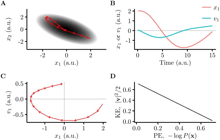
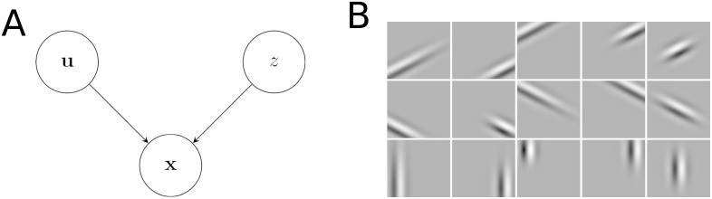
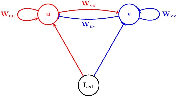
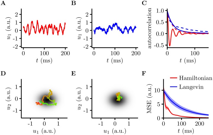
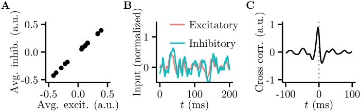
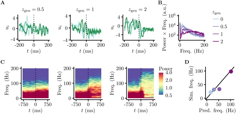
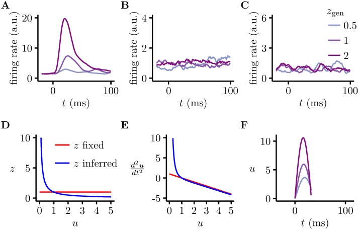
Probabilistic inference offers a principled framework for understanding both behaviour and cortical computation. However, two basic and ubiquitous properties of cortical responses seem difficult to reconcile with probabilistic inference: neural activity displays prominent oscillations in response to constant input, and large transient changes in response to stimulus onset. Indeed, cortical models of probabilistic inference have typically either concentrated on tuning curve or receptive field properties and remained agnostic as to the underlying circuit dynamics, or had simplistic dynamics that gave neither oscillations nor transients. Here we show that these dynamical behaviours may in fact be understood as hallmarks of the specific representation and algorithm that the cortex employs to perform probabilistic inference. We demonstrate that a particular family of probabilistic inference algorithms, Hamiltonian Monte Carlo (HMC), naturally maps onto the dynamics of excitatory-inhibitory neural networks. Specifically, we constructed a model of an excitatory-inhibitory circuit in primary visual cortex that performed HMC inference, and thus inherently gave rise to oscillations and transients. These oscillations were not mere epiphenomena but served an important functional role: speeding up inference by rapidly spanning a large volume of state space. Inference thus became an order of magnitude more efficient than in a non-oscillatory variant of the model. In addition, the network matched two specific properties of observed neural dynamics that would otherwise be difficult to account for using probabilistic inference. First, the frequency of oscillations as well as the magnitude of transients increased with the contrast of the image stimulus. Second, excitation and inhibition were balanced, and inhibition lagged excitation. These results suggest a new functional role for the separation of cortical populations into excitatory and inhibitory neurons, and for the neural oscillations that emerge in such excitatory-inhibitory networks: enhancing the efficiency of cortical computations.

Fig 1. An example of Hamiltonian dynamics.

A. Movement of a particle under Hamiltonian dynamics (i.e. with momentum) on a two-dimensional quadratic potential energy landscape (greyscale, darker means lower energy) corresponding to a multivariate Gaussian probability density. The red arrows show the trajectory, with each arrow representing an equal time interval. Note that the particle does not just go to the lowest potential energy location: it picks up momentum (kinetic energy) as it moves, leading it to oscillate around the energy well. B. A plot of position (red) and velocity (blue, the derivative of position) along one dimension. C. Plotting velocity and position directly against each other reveals explicitly that the dynamics of the system is similar to that of a harmonic oscillator. D. Plotting kinetic energy (KE) against potential energy (PE) reveals an exchange between kinetic energy and potential energy that contributes to the system’s oscillatory behaviour.

Fig 2

A. The graphical model representation of the Gaussian scale mixture model. The distribution over the observations (images), x, depends on two latent variables, z and u. The vector u represents the intensity of edge-like features (see panel B) in the images. The positive scalar z represents the overall contrast level in the image. B. The basis functions represented by u were 15 Gabor filters centred at five different locations, and with three different orientations.

Fig 3. The architecture of the Hamiltonian network.

The network consists of two populations of neurons, excitatory neurons with membrane potential u, and inhibitory neurons v, driven by external input I_input. Neurons in the network are recurrently coupled by synaptic weights, W_uu, W_uv, W_vu and W_vv. Red arrows represent excitation; blue bars represent inhibition.

Fig 4. The Hamiltonian sampler is more efficient than a Langevin sampler.

A, B. Example membrane potential traces for a randomly selected neuron in the Hamiltonian network (A) and the Langevin network (B). C. Solid lines: the autocorrelation of membrane potential traces in A and B, for Hamiltonian (red) and Langevin samplers (blue). Dashed lines: the autocorrelation of the joint (log) probability for Hamiltonian (red) and Langevin samplers (blue). Note that for the Hamiltonian sampler, the joint probability is over both u and v. D, E. Joint membrane potential traces from two randomly selected neurons in the Hamiltonian network (D) and the Langevin network (E), colour indicates time (from red to green, spanning 25 ms), grey scale map shows the (logarithm of the) underlying posterior (its marginal over the two dimensions shown). F. Normalised mean square error (MSE) between the true mean and the mean estimate from samples taken over a time t for the Langevin (blue) and Hamiltonian dynamics (red), with 100 repetitions (mean ± 2 s.e.m.).

Fig 5. Excitation and inhibition are balanced in the Hamiltonian network.

A. Trial-average excitatory input vs. trial-average inhibitory input across trials (dots) for a randomly selected individual cell in the network. B. Total inhibitory input to a single cell (blue) closely tracks but slightly lags total excitatory input (red) over the course of a trial. C. The cross-correlation between the average excitatory and average inhibitory membrane potentials shows a peak that is offset from 0 time.

Fig 6. Oscillation frequency depends on stimulus contrast.

A. The membrane potential response of one neuron to stimulus onset across 4 trials (coloured curves) shows that the variability decreases and the frequency increases as stimulus contrast increases. The true contrast of the underlying image increases left to right (z_gen = 0.5, 1, and 2). B. Power spectrum of the LFP (average membrane potentials) at different contrasts (coloured lines), showing that dominant oscillation frequency increases with contrast. Note that we plot power × frequency on the y-axis, in order to account for the fact that noise from a “scale-free” process has 1/f frequency dependence [59]. C. Time-dependent spectrum (Gaussian window, width 100 ms) of the LFP (contrast levels as in A). D. The simplified dynamics (x-axis, Eq 8) accurately predicted the dependence of oscillation frequencies on contrast (colour code as in B) in the full network (y-axis).

Fig 7. Large, contrast-dependent firing rate transients in the model.

A-C. Transients (or lack thereof) at different contrast levels (colour) under the full dynamics (A), using Langevin dynamics (B), and under the full dynamics when the value of z is fixed, z = z_gen (C). Note different scales for firing rates in the three panels to better show the full range of firing rate fluctuations in each case. D. Dependence of the inferred value of contrast, z, on the currently inferred magnitude of basis function intensities, u, under the simplified dynamics (blue). For reference, red shows the value of z when set to be fixed at z = z_gen. E. There is asymmetry in $\ddot{u}$ as a function of u, around the value of u = $\overline{u}$ = 1, in the simplified model when z is inferred (blue) but not when it is fixed (red). F. Transients predicted by the simplified dynamics (Eq 9, with parameters as in Fig 6D, and initial conditions u(0) = 0.1 and $\dot{u}\left(0\right)=0$) are similar to transients under the full dynamics.

References

1. Knill DC. Surface orientation from texture: ideal observers, generic observers and the information content of texture cues. Vision Research. 1998;38:1655–1682. 10.1016/S0042-6989(97)00324-6 - DOI - PubMed
1. Jacobs RA. Optimal integration of texture and motion cues to depth. Vision Research. 1999;39:3621–3629. 10.1016/S0042-6989(99)00088-7 - DOI - PubMed
1. van Beers RJ, Sittig AC, van der Gon JJD. Integration of proprioceptive and visual position-information: An experimentally supported model. Journal of Neurophysiology. 1999;81:1355–1364. - PubMed
1. Ernst MO, Banks MS. Humans integrate visual and haptic information in a statistically optimal fashion. Nature. 2002;415:429–433. 10.1038/415429a - DOI - PubMed
1. Wolpert DM, Ghahramani Z, Jordan MI. An internal model for sensorimotor integration. Science. 1995;269:1880–1880. 10.1126/science.7569931 - DOI - PubMed
LinkOut - more resources