Stable population coding for working memory coexists with heterogeneous neural dynamics in prefrontal cortex

Abstract

Working memory (WM) is a cognitive function for temporary maintenance and manipulation of information, which requires conversion of stimulus-driven signals into internal representations that are maintained across seconds-long mnemonic delays. Within primate prefrontal cortex (PFC), a critical node of the brain's WM network, neurons show stimulus-selective persistent activity during WM, but many of them exhibit strong temporal dynamics and heterogeneity, raising the questions of whether, and how, neuronal populations in PFC maintain stable mnemonic representations of stimuli during WM. Here we show that despite complex and heterogeneous temporal dynamics in single-neuron activity, PFC activity is endowed with a population-level coding of the mnemonic stimulus that is stable and robust throughout WM maintenance. We applied population-level analyses to hundreds of recorded single neurons from lateral PFC of monkeys performing two seminal tasks that demand parametric WM: oculomotor delayed response and vibrotactile delayed discrimination. We found that the high-dimensional state space of PFC population activity contains a low-dimensional subspace in which stimulus representations are stable across time during the cue and delay epochs, enabling robust and generalizable decoding compared with time-optimized subspaces. To explore potential mechanisms, we applied these same population-level analyses to theoretical neural circuit models of WM activity. Three previously proposed models failed to capture the key population-level features observed empirically. We propose network connectivity properties, implemented in a linear network model, which can underlie these features. This work uncovers stable population-level WM representations in PFC, despite strong temporal neural dynamics, thereby providing insights into neural circuit mechanisms supporting WM.

Keywords: population coding; prefrontal cortex; working memory.

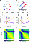
Fig. 1.

WM tasks and PFC population dynamics. (A) In the ODR task, the subject fixates on a central point, and a visuospatial cue of variable spatial angle is presented for 0.5 s, followed by a 3-s mnemonic delay. After the delay, the subject makes a saccadic eye movement to the remembered location (14). (B) In the VDD task, the subject receives a 0.5-s vibrotactile stimulus of variable mechanical frequency (cue, f1) to the finger, followed by a 3-s mnemonic delay. After the delay, a second stimulus (f2) is presented and the subject reports, by level release, which stimulus had a higher frequency (15). (C and D) Correlation between population states as a function of time, within the same stimulus condition. The sensory state is defined by the first 0.25 s of the cue epoch and the late memory state by the last 0.25 s of the delay epoch. Colored shaded regions mark SEM. (E and F) Correlation between the population states at different timepoints (i.e., time-lagged autocorrelation). The correlation between states is generally high due to a broad distribution of overall firing rates across neurons (Fig. S2). The traces in C and D are slices along the corresponding timepoint.

Fig. S1.

Example single neurons, for ODR (A1–A6) and VDD (B1–B6) datasets, highlighting the heterogeneity and temporal dynamics in single-neuron activity in PFC during WM encoding and maintenance. Plotted is the PSTH for each stimulus condition, with trace colors marking the different stimulus conditions corresponding to those shown in the task schematics of Fig. 1. The gray shaded region marks the cue epoch. Purely for visualization of example single-neuron activity in this figure only, PSTHs were smoothed using PCA, which denoises across PSTH traces rather than only over time. For all reported results, activity is not smooth in any way except for binning in 0.25-s time bins.

Fig. S2.

Distribution of mean firing rates across neurons in different task epochs. (A and B) Firing-rate distributions plotted in a lin-log plot, with logarithmic x axis and linear y axis. The observed distribution of firing rates is approximately a log-normal distribution. Interestingly, when compared across task epochs (foreperiod, cue, working memory delay), the overall distribution of firing rates does not change substantially. In particular, the distribution during the delay epoch is essentially the same as during the foreperiod. (C and D) Correlation across neurons of mean firing rates between task epochs. Shown here are the correlations between delay epoch and the foreperiod epoch. The values of the Pearson’s r correlation coefficient of the log-transformed firing rates are the following: For ODR, 0.88 for foreperiod–cue, 0.91 for foreperiod–delay, and 0.89 for cue–delay; for VDD, 0.75 for foreperiod–cue, 0.83 for foreperiod–delay, and 0.66 for cue–delay.

Fig. S3.

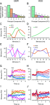
PCA of time-averaged delay activity. (A and B) Amount of stimulus variance captured by each principal axis, for time-averaged delay activity. The number of PCs is one fewer than the number of stimulus conditions. Stimulus variance captured is normalized by the number of neurons. Gray error bars show the mean and central 95% bounds, calculated through shuffling the stimulus identities of trials. For the ODR dataset, a subspace defined by the first two principal axes captures 68% of the stimulus variance. For the VDD dataset, a subspace defined by the first principal axis captures 60% of the stimulus variance. (C and D) Leading PCs, i.e., projections of the time-averaged delay activity along the leading principal axes (2 for ODR, 1 for VDD). For ODR (C), PC1 and PC2 provide quasi-sinusoidal coding of stimuli. For VDD (D), PC1 provide quasi-linear coding of stimuli. (E and F) Projections along the next two leading principal axes. (G and H) Population trajectory projected along principal axis 1, showing relative stability of stimulus coding during the delay epoch as well as in the preceding cue epoch. (I and J) Population trajectory projected along principal axis 2.

Fig. 2.

Stable population coding of WM coexists with strong temporal dynamics. (A and B) Population trajectories during the WM delay epoch projected into the mnemonic subspace, defined via PCA on time-averaged delay activity. Here the x and y axes show the first and second principal components (PC1 and PC2) of the subspace. Each trace corresponds to a stimulus condition, colored as in Fig. 1 A and B. The shading of the traces marks the time during the delay, from early (light) to late (dark). (C and D) Three-dimensional projections, illustrating the strong temporal dynamics coexisting with stable coding in the mnemonic subspace. The x and y axes are as in A and B. The z axis (time PC1) is an orthogonal axis in the state space that captures time-related activity variance, but does not indicate time explicitly. Within each plot, all axes are scaled equally.

Fig. S4.

Stimulus- and time-related variance of delay activity captured by the mnemonic subspace, for each dimension in the mnemonic subspace. (A and B) The green points show the variance (per neuron), across stimuli, for the time-averaged mean delay activity, i.e., $\frac{1}{N}{\text{Var}}_s({\text{Mean}}_t(𝐫(s,t))$. The orange points show the average within-stimulus, time-related variance (per neuron) of the trajectory (using 0.25-s time bins), i.e., $\frac{1}{N}{\text{Mean}}_s({\text{Var}}_t(𝐫(s,t))$. The orange points may overestimate the true time-related variance, as variance will be contributed by noisy estimation of the PSTH due to finite numbers of trials. Error bars denote the 95% range generated by leave-one-neuron-out jackknife resampling, characterizing how much these estimates would change if additional neurons were included.

Fig. 3.

Stimulus variance captured by the mnemonic and dynamic coding subspaces. The mnemonic subspace is defined using delay activity as in Fig. 2. The dynamic subspace is defined from data for each timepoint (0.25 s). The dimensionality of the subspaces is 2 for ODR (A and C) and 1 for VDD (B and D), matching the dimensionality of the stimulus feature for each task. (A and B) Stimulus variance captured for stable mnemonic subspace (blue) and for a dynamic subspace optimized for each timepoint (red). Chance values for the stable (gray) and dynamic (brown) subspaces were calculated by shuffling stimulus trial labels. (C and D) Generalizability of the dynamic subspace across time. The red curve marks the stimulus variance captured by the dynamic subspace defined at one time for activity at another time separated by a given time separation, averaged across timepoints during the delay. The blue dashed line marks the stimulus variance captured by the mnemonic subspace, averaged across the delay epoch. The gray dotted line marks the mean chance level during the delay. Shaded bands mark SEM.

Fig. S5.

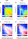
Stimulus variance captured by mnemonic and dynamic subspaces and generalizability of the dynamic subspace. (A and B) Stimulus variance captured by the dynamic subspace as a function of the training timepoint and testing point. That is, activity at the training time is used to define the dynamic subspace, and the activity at the testing time is projected into that subspace. The diagonal elements, when training time and testing time are the same, are plotted in the Fig. 3 A and B. (C and D) The relative difference in stimulus variance captured for dynamic vs. mnemonic subspaces ($V_{dyn}$ and $V_{mne}$, respectively), as a function of training time and testing time during the cue and delay epochs. That is, the value plotted is $z(t_i,t_j)=V_{dyn}(t_i,t_j)/V_{mne}(t_j)$. Red (blue) regions show where the dynamic subspace has higher (lower) stimulus variance captured than the mnemonic subspace. These results show that the dynamic subspace classifier does not generalize well, so that for off-diagonal elements when training time and testing time are separated by more than 0.5 s, the mnemonic subspace shows greater performance. This characterizes the timescales of dynamic coding. Color bars have a logarithmic scale.

Fig. 4.

Decoding of stimulus via stable and dynamic coding subspaces. (A and B) Schematic of the subspace decoder. Activity at a given timepoint for a single trial is projected into the subspace, and the classifier’s winner-take-all readout is the stimulus condition whose centroid is nearest ($d_{min}$). As in Fig. 3, the number of dimensions used for the subspace is 2 for ODR and 1 for VDD. (C and D) Decoding accuracy over time for the mnemonic (blue) and dynamic (red) coding subspaces. Chance performance for the stable (gray) and dynamic (brown) subspaces was calculated by shuffling stimulus trial labels. (E and F) Generalizability of the dynamic subspace across time. The red curve marks the stimulus variance captured by the dynamic subspace defined at one time for activity at another time separated by a given time separation, averaged across timepoints during the delay. The blue dashed line marks the stimulus variance captured by the mnemonic subspace, averaged across the delay epoch. The gray dotted line marks chance performance. Shaded bands mark SEM.

Fig. S6.

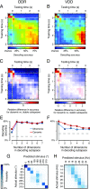
Decoding performance for a nearest-mean classifier based on mnemonic or dynamic subspaces. (A and B) Decoding accuracy and generalizability of the dynamic subspace classifier as a function of the training timepoint and testing point. The diagonal elements, when training time and testing time are the same, are plotted in Fig. 4 B and C. (C and D) The relative difference in stimulus variance captured for dynamic vs. mnemonic subspaces ($P_{dyn}$ and $P_{mne}$, respectively), as a function of training time and testing time during the cue and delay epochs. That is, the value plotted is $z(t_i,t_j)=(P_{dyn}(t_i,t_j)-P_{mne}(t_j))/P_{mne}(t_j)$. Red (blue) regions show where the dynamic subspace has higher (lower) decoding accuracy than the mnemonic subspace. These results show that the dynamic subspace outperforms the mnemonic subspace most during the cue and early delay epochs. Furthermore, the dynamic subspace classifier does not generalize well, so that for off-diagonal elements when training time and testing time are separated by more than 0.5 s, the mnemonic subspace shows greater performance. (E and F) Decoding accuracy as a function of the number of dimensions included in the decoding subspace. A $k$-dimensional decoding subspace is defined by the leading $k$ principal components. The gray dashed lines mark chance performance. In C and D the gray shaded line marks the number of dimensions used for each dataset, 2 for ODR and 1 for VDD, which matches the dimensionality of the stimulus. The decoding accuracy can plateau or decline with increasing dimensionality, because adding another dimension not only increases signal but also increases trial-by-trial variability that can impair classifier performance. (G and H) Confusion matrix characterizing the pattern of errors made by the mnemonic subspace classifier. The confusion matrix shows the distribution of classifier predictions for the stimulus condition (columns) for each actual stimulus condition (rows). For both ODR and VDD, the classification errors (off-diagonal elements of the confusion matrix) are primarily made to stimuli that are near actual stimulus. (G) For ODR, most errors are due to the compressed representation of ipsilateral space, which produces poor separation among the three left hemifield stimuli (135°, 180°, and 225°). (H) For VDD, most errors are to adjacent stimuli, and the predicted stimulus is biased toward more central stimulus values.

Fig. 5.

Population-level analyses measures distinguish theoretical model network mechanisms for population coding and dynamics. We tested four dynamical circuit models, described in the main text: stable attractor, feedforward chain, chaotic random, and stable subspace. The simulated stimulus features are designed to match the ODR task. (A) Example activity for one neural unit in the network. Each colored trace indicates a different stimulus condition, as for ODR. (B) Correlation of population state as a function of time, as in Fig. 1 C and D. We show the correlation for each timepoint with the sensory (orange) and late memory (purple) states. (C) Delay-activity state–space trajectories, as in Fig. 2 C and D. (D) Stimulus variance captured over time, for mnemonic (blue) and dynamic (red) coding subspaces, as in Fig. 3 A and B.

References

1. Goldman-Rakic PS. Cellular basis of working memory. Neuron. 1995;14(3):477–485. - PubMed
1. Wang XJ. Synaptic reverberation underlying mnemonic persistent activity. Trends Neurosci. 2001;24(8):455–463. - PubMed
1. Compte A, Brunel N, Goldman-Rakic PS, Wang XJ. Synaptic mechanisms and network dynamics underlying spatial working memory in a cortical network model. Cereb Cortex. 2000;10(9):910–923. - PubMed
1. Machens CK, Romo R, Brody CD. Flexible control of mutual inhibition: A neural model of two-interval discrimination. Science. 2005;307(5712):1121–1124. - PubMed
1. Shafi M, et al. Variability in neuronal activity in primate cortex during working memory tasks. Neuroscience. 2007;146(3):1082–1108. - PubMed
Publication types