Asymmetric unwrapping of nucleosomal DNA propagates asymmetric opening and dissociation of the histone core

Abstract

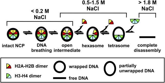
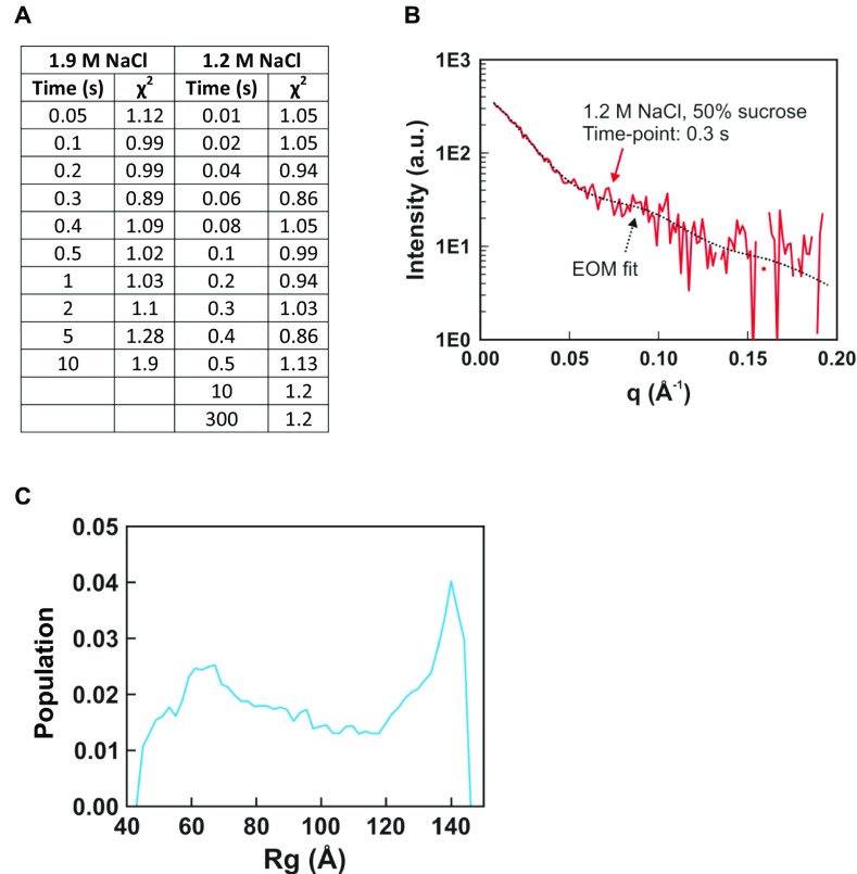
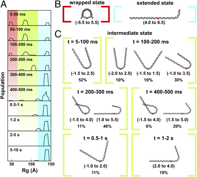
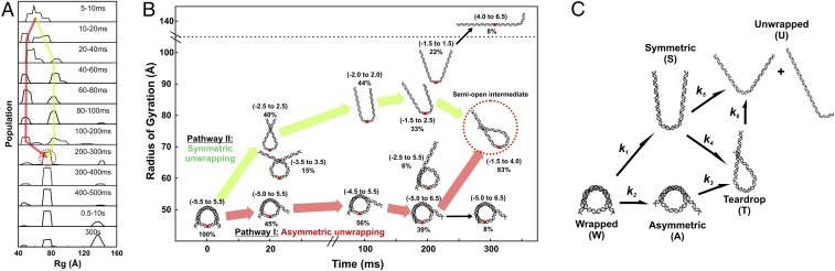
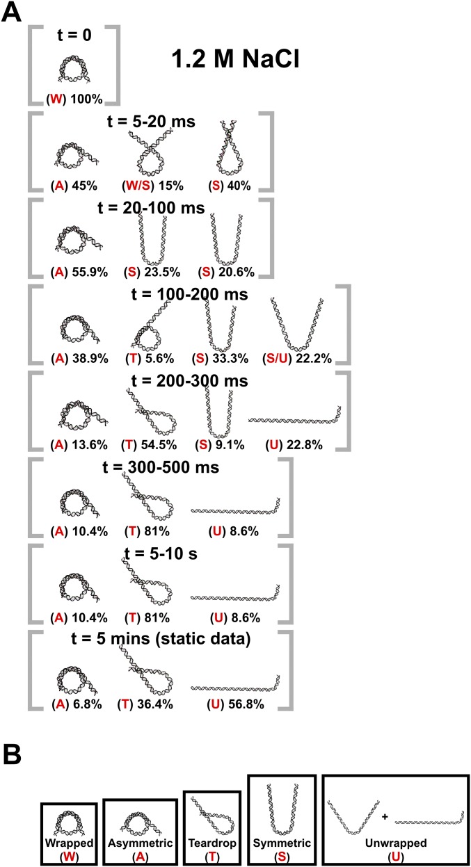
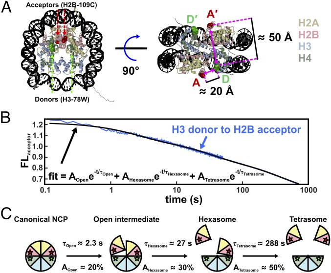
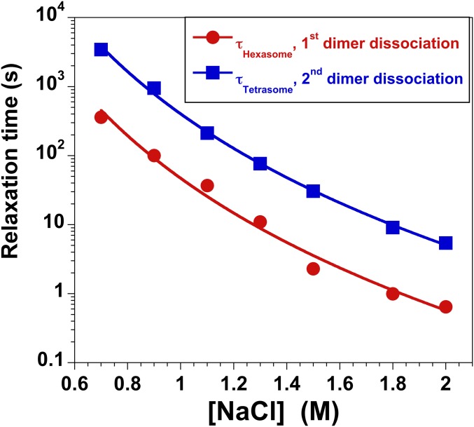
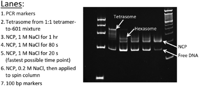
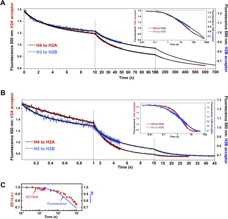
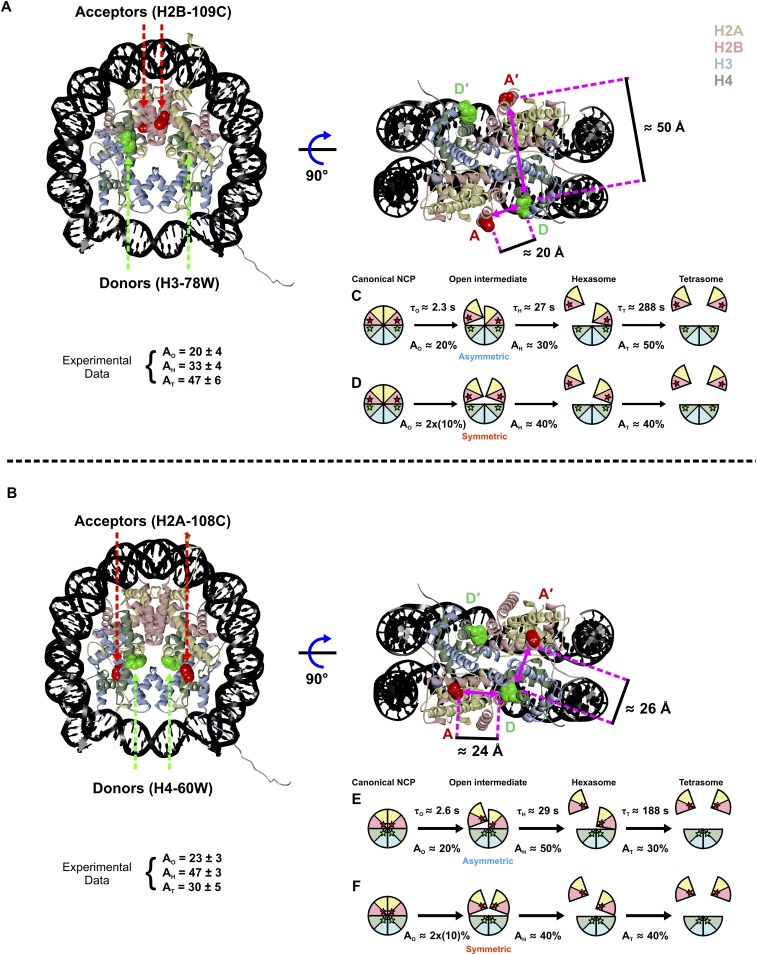
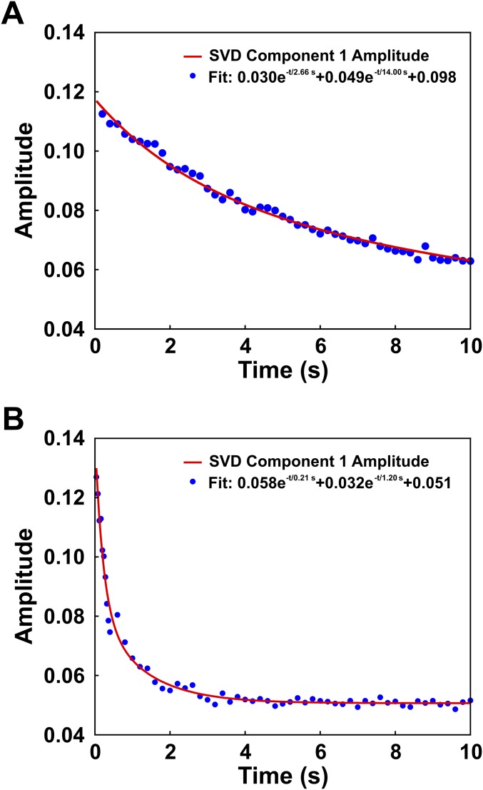
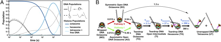
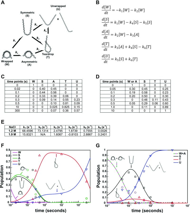
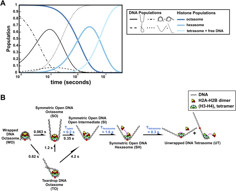
The nucleosome core particle (NCP) is the basic structural unit for genome packaging in eukaryotic cells and consists of DNA wound around a core of eight histone proteins. DNA access is modulated through dynamic processes of NCP disassembly. Partly disassembled structures, such as the hexasome (containing six histones) and the tetrasome (four histones), are important for transcription regulation in vivo. However, the pathways for their formation have been difficult to characterize. We combine time-resolved (TR) small-angle X-ray scattering and TR-FRET to correlate changes in the DNA conformations with composition of the histone core during salt-induced disassembly of canonical NCPs. We find that H2A-H2B histone dimers are released sequentially, with the first dimer being released after the DNA has formed an asymmetrically unwrapped, teardrop-shape DNA structure. This finding suggests that the octasome-to-hexasome transition is guided by the asymmetric unwrapping of the DNA. The link between DNA structure and histone composition suggests a potential mechanism for the action of proteins that alter nucleosome configurations such as histone chaperones and chromatin remodeling complexes.

Keywords: FRET; contrast variation SAXS; hexasome; nucleosomes; time resolved.

Fig. 1.

A schematic of NaCl-dependent disassembly for NCPs containing the 601-DNA (15), based on equilibrium studies ([NCP] ≥ 25 nM). At physiological ionic strength, NCP configurations reflect local dynamics [i.e., DNA breathing (6), and formation of an open intermediate (8)]. Above 0.5 M NaCl, H2A–H2B dimers begin to dissociate, allowing the formation of hexasomes and tetrasomes (23). Above 1.4 M NaCl, (H3–H4)₂ tetramers begin to dissociate, allowing for complete disassembly (24). Although dimer dissociation is reversible, tetrasomes are the minimal configurations required to maintain a wrapped DNA structure.

Fig. 2.

Contrast variation SAXS isolates structural information for the DNA component of NCPs. (A) Color scale bar with typical electron density values for solvent (water), protein, and DNA. (B and C) NCP structures (PDB 1AOI) shown in buffers with electron densities that vary depending on the presence of 0% (B) or 50% (C) sucrose. We used contrast variation SAXS to monitor DNA conformations during NCP disassembly induced with a salt jump.

Fig. S1.

Time-resolved SAXS profiles for NCPs destabilized by NaCl in 50% sucrose. (A and B) Time course measured for NCPs in 1.9 M NaCl (A) and 1.2 M NaCl (B). SAXS profiles for the time points after 0.5 s were collected using an attenuated X-ray beam to reduce the effects of radiation damage. Similar signal-to-noise ratios were achieved for the data collected within each salt series by using longer time bins (1 s) for the time points collected with the attenuator (for details, see Materials and Methods). SAXS profiles were offset for enhanced visualization and negative values are not shown on the log plot.

Fig. 3.

Overview of the ensemble optimization method (EOM) used for determining structures. Ensemble optimization (step 3, red box) requires SAXS profiles (step 1) and a pool of DNA structures (step 2) that contains a large number of possible conformations. First, the theoretical SAXS profile for each structure in the pool is calculated using CRYSOL (step 3, Left). A genetic algorithm (GAJOE) randomly selects subsets of these structures, called ensembles, for comparison with the input SAXS data (step 3, Right). Structures from the best-fitting ensembles are propagated into the next generation of ensembles along with some new structures, and this process is repeated (10,000 times) until convergence is achieved. The entire ensemble optimization process is repeated (100 times) to confirm reproducibility and the final ensembles that best represent the data are used to generate histograms of the radius of gyration and to determine the most representative structures for the SAXS profiles (step 4). The example fit and results shown are for the 300-ms time point of NCPs in 1.2 M NaCl under contrast-matched conditions (proteins “invisible” in 50% sucrose).

Fig. S2.

Ensemble optimization method (EOM) analysis of TR-SAXS data. (A) Table of χ² values for EOM fits to TR-SAXS data. (B) Representative fit of SAXS profile calculated for the ensemble of structures selected by EOM that best recapitulate the measured TR-SAXS profile. (C) Histogram of radius of gyration (Rg) values for the DNA pool (9,182 structures) used for EOM analysis. The Rg histograms for the time course of selected ensembles are shown in Figs. 4A and 5A. The pool of DNA structures used in this study was sufficiently large enough to create ensembles of structures that fit the data well.

Fig. 4.

DNA structures selected by EOM analysis of TR-SAXS data for NCPs dissociated in 1.9 M NaCl and 50% sucrose. (A) Rg(t) histograms for DNA structural models selected by EOM. Regions highlighted in red, green, and blue correspond with the fully wrapped, intermediate, and extended states, respectively. (B) Models that best represent the measured SAXS profile for the initial wrapped state (red) and final extended state (blue). (C) Models that best represent the intermediate states as a function of time. Red dots indicate the dyad axis or superhelical location zero (SHL 0). Numbers in the parentheses reveal the range of SHLs (number of turns where the major groove faces the histone, every 10 bp) contained within the curved portions. Percentages show the weights of the species out of the total population at the indicated time point. Under high-salt conditions where complete dissociation of 601-NCPs is favored, multiple partially unwrapped intermediates are populated.

Fig. 5.

DNA structures selected by EOM for NCPs dissociated in 1.2 M NaCl. (A) Rg histograms from DNA models selected by EOM that best represent the SAXS data. Red and green arrows highlight two pathways through which DNA structures change before settling into a prominent peak after 300 ms (circled in red). (B) DNA models selected by EOM before (t = 0) and after mixing into 1.2 M NaCl (20 ms, 100 ms, 200 ms, and 300 ms). Green and red arrows highlight two major pathways through which DNA unwraps to form the teardrop DNA structure. Black arrows show minor pathways. Red dots indicate the dyad axis (SHL 0). Numbers in parentheses reveal the range of SHLs (number of turns) contained within the curved portions. Percentages shown are the weights of the species out of the total population at the indicated time point. Under moderate salt conditions that favor partial disassembly, the majority of structures unwrap symmetrically and asymmetrically before converging into the teardrop structure. (C) Kinetic scheme for complete disassembly with pathways inferred from prominent DNA structures selected by EOM (Fig. S3).

Fig. S3.

Ensembles of DNA structures selected by EOM. (A) DNA structures selected for NCPs in 1.2 M NaCl as a function of time. Percentages shown are the weights of the species out of the total population at the indicated time point. (B) Generalized classes of DNA conformations into which the models selected by EOM were grouped. The red letters for each model in A designate how the structures were grouped for subsequent analysis. Multiple letters mean that the population weight was split between the reported classes.

Fig. 6.

NCP FRET pairs and the histone configurations observed. (A) FRET pairs with H3-78W donor (green) and H2B-109CysAEDANS acceptor (red). For this construct (H3–H2B NCP), the donor and acceptor on the same face of the NCP (D–A) are close to the Förster radius for this FRET pair (∼20 Å), but the distance from the donor to the acceptor on the other NCP face (D–A′) is significantly longer (∼50 Å) and should contribute less than 1% to the observed FRET signal. The Cβ positions in the 1AOI.pdb structure of the NCP were used to estimate distances between the FRET pairs. (B) Acceptor fluorescence time course measured for 250 nM NCP in 1.2 M NaCl (blue). The solid black line represents a sum of three first-order exponentials used to determine the relative amplitudes and relaxation times. To obtain robust values, global fits were used on datasets collected as a function of NCP concentration (10–250 nM NCP). (C) Histone configurations observed with TR-FRET. Relaxation times (τ) and amplitudes (A) of FRET loss measured at 1.2 M NaCl are reported for each transition.

Fig. S4.

Salt dependence of the kinetic responses measured by FRET using the H3-78W/H2B-109CA donor–acceptor pair. Dissociation was initiated primarily by manual mixing methods, with a time resolution of ∼2 s. However, at NaCl concentrations of ≥1.5 M, the more rapid kinetic response was also determined using stopped-flow mixing, with a time resolution of ∼10 ms. Multiple kinetic traces at a given salt concentration were globally fit to a sum of two exponentials, yielding relaxation times τ_hexasome (red circles) and τ_tetrasome (blue squares) describing the dissociation of the first and second H2A–H2B dimers, respectively. The errors associated with the relaxation times are equal to or smaller than the size of the symbols. The lines are drawn to guide the eye and do not reflect a mechanistic fit of the data. Final conditions were as follows: 25 nM NCP, 20 mM Tris-Cl (pH 7.5), 0.1 mM EDTA, 0.1 mM DTT, 25 °C.

Fig. S5.

Gel assay for salt-induced dissociation of NCPs. Native gels for desalted NCPs incubated with NaCl for varying amounts of time show the timescales upon which hexasomes and tetrasomes are formed. Any amount of NaCl leads to the presence of a free DNA band on the gel (a technical artifact). These results qualitatively show that the hexasome is formed on the timescale of 20–80 s, with even slower formation of the tetrasome.

Fig. S6.

Representative FRET responses for NCPs destabilized by NaCl. (A) Acceptor fluorescence time course measured for NCPs in 1.2 M NaCl. Each dataset (averaged over 20 kinetic measurements) shows the decrease in acceptor fluorescence after initiation of the salt jump for each FRET construct used. The final NCP concentration was 250 nM NCP. (B) Same as A, except NCPs were measured in 1.9 M NaCl. The solid black lines represent the global fits to a sum of three first-order exponentials for datasets collected as a function of NCP concentration (10–250 nM NCP). The relaxation times and relative amplitudes derived from these fits are reported in Table 1. Insets in A and B are log scale presentations of time courses. (C) Comparison of relative TR-FRET changes with I(0,t) measured using TR-SAXS for NCPs in 0% sucrose and 1.2 M NaCl. The dynamics measured on overlapping timescales agree well between SAXS and FRET.

Fig. S7.

Models of dimer dissociation reported by two different FRET pairs. (A and B) NCP structure (1AOI) highlighting the distances between the FRET pairs: H3-78W donor to H2B-109CA acceptor (H3–H2B NCP) (A) and H4-80W donor to H2A-108CA acceptor (H4–H2A NCP) (B). Due to the symmetry of the structures in both constructs, distances are mirrored between the FRET pairs on both sides. Note: The Förster radius R₀ ∼20 Å. The distances for the D–A pair (on the same NCP face) and D–A′ pair (across the NCP) are similar for the H4–H2A NCP. Although equal changes in FRET signals are expected for the D–A and D–A′ interactions, the dissociation of a single H2A–H2B dimer should still be reflected by the loss of ∼50% of the FRET signal due to the symmetry of the construct. Below each model in A and B are the measured FRET amplitudes (as reported in Table 1). (C–F) Models of possible histone configurations to explain the amplitude patterns observed for H3–H2B NCP (C and D) and H4–H2A NCP (E and F). For each FRET pair, the expected amplitude changes are shown for the scenarios that the open intermediate is formed asymmetrically (C and E) and symmetrically (D and F). The measured amplitude patterns differ between H3–H2B NCP (33% → 47%) and H4–H2A NCP (47% → 30%). Release of the first H2A–H2B dimer may slightly destabilize the remaining H2A–H2B dimer (depicted as a slight separation) through the loss of some minor contacts between the two H2A–H2B dimers. The H4–H2A NCP construct may be more sensitive to this destabilization due to the positions of the FRET pair. Our data are most consistent with the sequential formation as follows: canonical NCP → asymmetric open intermediate → hexasome → tetrasome.

Fig. S8.

Determination of relaxation times using singular value decomposition (SVD) analysis of the full time course of SAXS profiles. The time-dependent amplitude of the first component is shown for NCPs measured in 0% sucrose and 1.2 M NaCl (A) and 1.9 M NaCl (B). The amplitude dynamics of the first component represents the largest changes observed in the SAXS profiles. These changes correspond with NCP disassembly and reflect both conformational changes as well as changes in molecular mass [changes in the forward scattering, I(0)]. The decreasing amplitudes were fit to sums of exponential decays as shown. The relaxation times observed here are remarkably consistent with the values determined from FRET as shown in Table 1.

Fig. 7.

TR-FRET and TR-SAXS analyses reveal hexasome formation at 1.2 M NaCl. (A) Predicted populations of DNA conformational states (black lines) and histone configuration states (blue lines) based on the kinetic rates determined for NCPs at 1.2 M NaCl from the kinetic analysis of EOM models (Figure 6A, see details in Fig. S9) and TR-FRET measurements (Table 1), respectively. (B) NCP disassembly pathway determined from TR-SAXS with histone configurations informed by TR-FRET. Black numbers reflect the SAXS relaxation times (inverse of rates in Fig. S9C). Blue numbers reflect the FRET relaxation times (Table 1). The curved black arrow represents a minor pathway. For simplicity, histone orientations were centered on the dyad when possible.

Fig. S9.

Calculation of kinetic rates from structures selected by EOM. (A) Kinetic scheme with pathways inferred from prominent DNA structures selected by EOM analysis for NCP data collected in 50% sucrose and 1.2 M NaCl (DNA structures selected at 1.9 M NaCl were nearly identical). (B) Kinetic equations describing the population dynamics for the kinetic scheme in A. (C) Time course of DNA structure populations determined from EOM analysis for NCP data collected with 50% sucrose and 1.2 M NaCl. (D) Same as C, except using results for 1.9 M NaCl. (E) Rates for the kinetic scheme in A determined by solving the kinetic equations in B using population data for NCPs in 1.2 M (C) and 1.9 M (D) NaCl. Note: Convergent solutions were achieved using the same kinetic scheme for both datasets, suggesting that the overall structures through which DNA unwraps are similar at both salt concentrations. However, the rates determined are quite different between these two conditions and indicate that not only is unwrapping faster at higher salt, but different pathways are preferred depending on [NaCl]. The opposite sign of k₄ at 1.9 M NaCl suggests that the symmetric unwrapped DNA is preferred over the teardrop at the more destabilizing condition. (F) Population data in C plotted with the simulated populations (lines) determined from the solved kinetic equations for 1.2 M NaCl (E). (G) Same as F, except using results for 1.9 M NaCl (D and E). Note: the asymmetrically unwrapped DNA state (A) was not observed sufficiently enough in 1.9 M NaCl to be reliably fit; thus it was not included in the fitting and k₂ and k₃ are linked together.

Fig. S10.

Predicted populations and kinetic pathway of salt-induced NCP dissociation in 1.9 M NaCl. (A) Predicted populations of DNA conformational states (black lines) and NCP oligomerization states (blue lines) based on the kinetic rates determined from EOM analysis (Fig. S9) and TR-FRET measurements (Table 1), respectively. (B) Kinetic models of salt-induced NCP dissociation in 1.9 M NaCl. The DNA conformations, associated pathways, and relaxation times (black numbers) were deduced from the SAXS EOM analysis (Fig. 4). For each DNA conformation, the oligomeric state of the histone core was deduced from the lifetime of the hexasome and tetrasome populations (A). The relaxation times for dimer dissociation (blue numbers) were measured by TR-FRET (Table 1). For simplicity, histone orientations were centered on the dyad when possible. In 1.9 M NaCl, the majority of the DNA unwraps from both ends simultaneously, followed by dimer dissociation.

References

1. Andrews AJ, Luger K. Nucleosome structure(s) and stability: Variations on a theme. Annu Rev Biophys. 2011;40:99–117. - PubMed
1. Luger K, Mäder AW, Richmond RK, Sargent DF, Richmond TJ. Crystal structure of the nucleosome core particle at 2.8 A resolution. Nature. 1997;389(6648):251–260. - PubMed
1. Bell O, Tiwari VK, Thomä NH, Schübeler D. Determinants and dynamics of genome accessibility. Nat Rev Genet. 2011;12(8):554–564. - PubMed
1. Luger K. Dynamic nucleosomes. Chromosome Res. 2006;14(1):5–16. - PubMed
1. Tims HS, Gurunathan K, Levitus M, Widom J. Dynamics of nucleosome invasion by DNA binding proteins. J Mol Biol. 2011;411(2):430–448. - PMC - PubMed
Publication types