Automated Quality Assessment of Structural Magnetic Resonance Brain Images Based on a Supervised Machine Learning Algorithm

Abstract

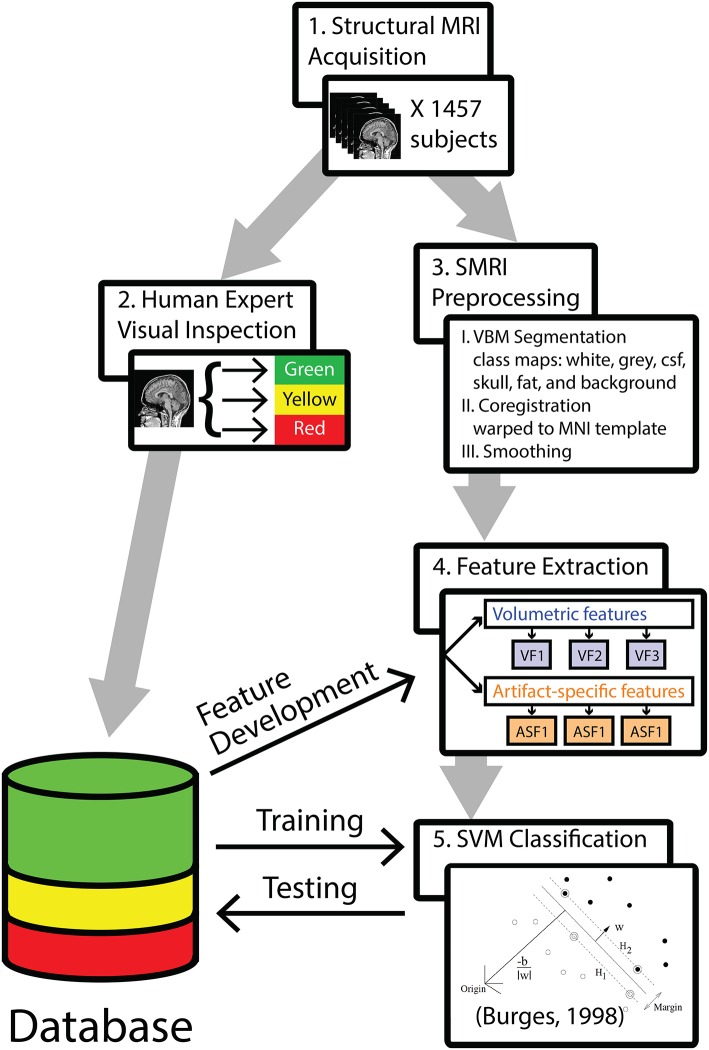
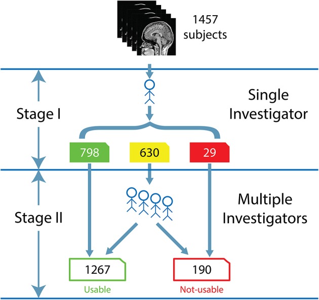
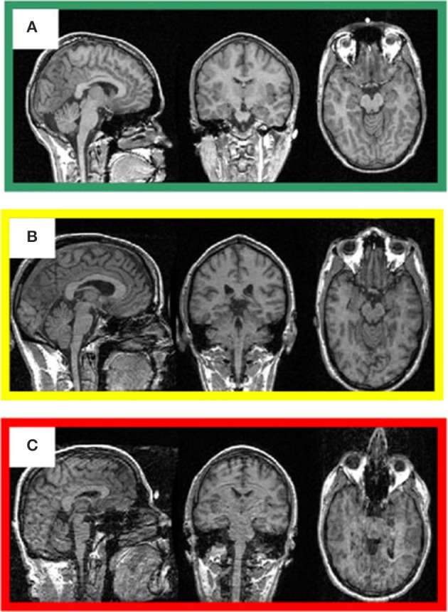
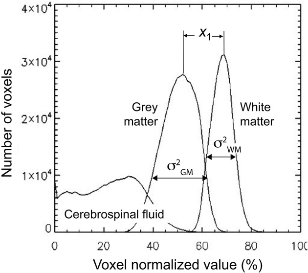
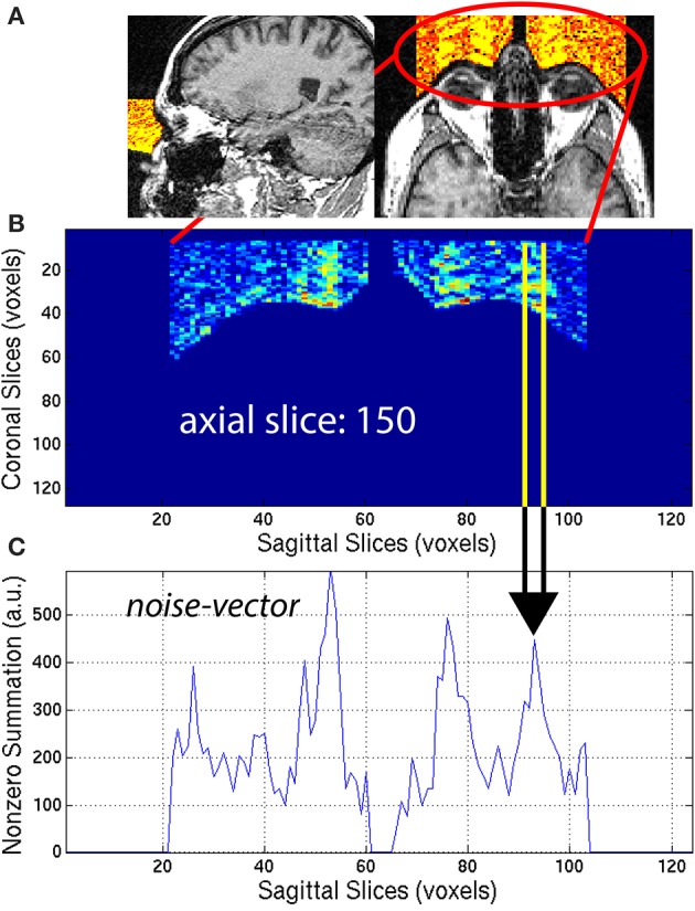
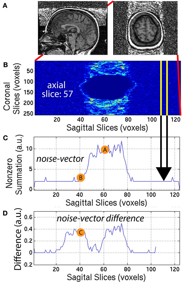
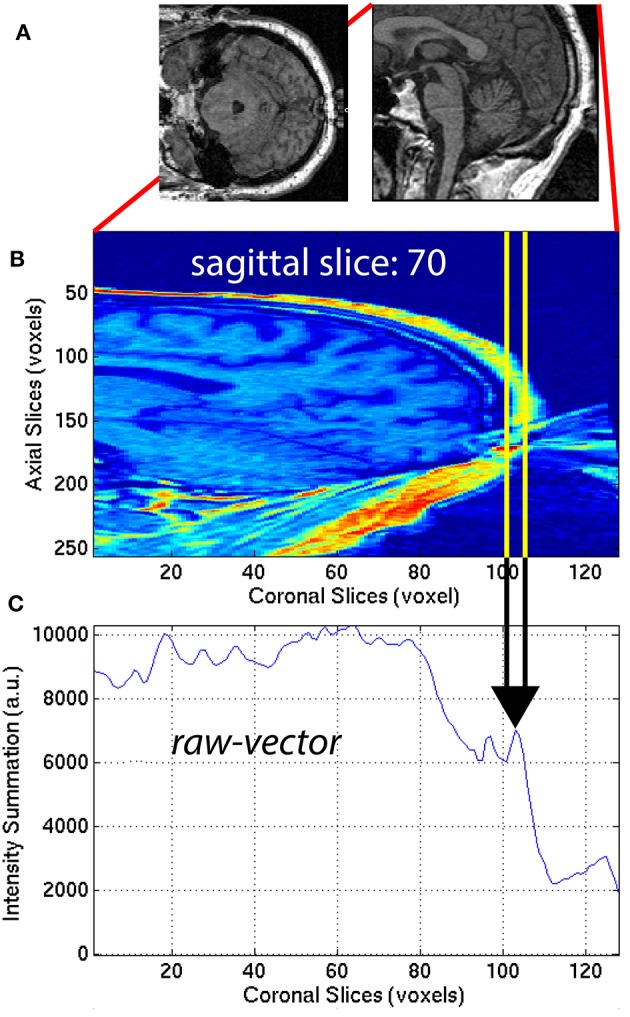
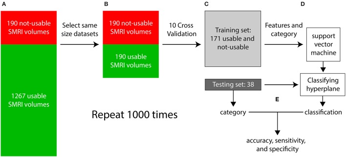
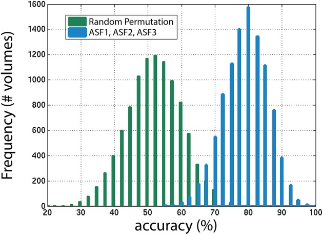
High-resolution three-dimensional magnetic resonance imaging (3D-MRI) is being increasingly used to delineate morphological changes underlying neuropsychiatric disorders. Unfortunately, artifacts frequently compromise the utility of 3D-MRI yielding irreproducible results, from both type I and type II errors. It is therefore critical to screen 3D-MRIs for artifacts before use. Currently, quality assessment involves slice-wise visual inspection of 3D-MRI volumes, a procedure that is both subjective and time consuming. Automating the quality rating of 3D-MRI could improve the efficiency and reproducibility of the procedure. The present study is one of the first efforts to apply a support vector machine (SVM) algorithm in the quality assessment of structural brain images, using global and region of interest (ROI) automated image quality features developed in-house. SVM is a supervised machine-learning algorithm that can predict the category of test datasets based on the knowledge acquired from a learning dataset. The performance (accuracy) of the automated SVM approach was assessed, by comparing the SVM-predicted quality labels to investigator-determined quality labels. The accuracy for classifying 1457 3D-MRI volumes from our database using the SVM approach is around 80%. These results are promising and illustrate the possibility of using SVM as an automated quality assessment tool for 3D-MRI.

Keywords: artifact detection; automated quality assessment; database management; machine learning; region of interest; structural magnetic resonance imaging; support vector machine.

Figure 1

A methods flowchart is presented to illustrate an overview of the steps involved in classifying structural 3D-MRIs in an automated fashion.

Figure 2

The flow for the human visual inspection procedure was realized for all 1457 datasets, is illustrated above and comprises of 2 Stages: (I) Visual inspection is performed by a single investigator to label the 3D-MRI volumes as green, yellow, or red. (II) Five to nine investigators then meet to further categorize the yellow 3D-MRI volumes as either usable or not-usable.

Figure 3

Representative 3D-MRI volumes are presented with corresponding image quality. (A) Green indicates usable and has excellent contrast between gray and white matter. (B) Volume contains slight ringing, was labeled yellow at stage I and usable at stage II. (C) Red indicates not-usable, has ringing, eye, and head movement.

Figure 4

The gw_t_score feature (VF3) is computed from the distribution of the gray and white matter class map histogram. The difference in means of the two distributions is estimated to be x₁ and the variance for each distribution is estimated as ${\sigma }_{GM}^2$ and ${\sigma }_{WM}^2$. These estimates are used to compute the gw_t_score given in Equation (4).

Figure 5

(A) An eye-mask is illustrated for a representative subject with noticeable eye movement artifact. (B) Each axial slice of the eye-mask was collapsed into a (C) noise-vector. The noise-vector is equal to the median, non-zero voxel of each column of voxels of the eye-mask, as in Equation (8). The feature ASF1 was computed as the max of the sum of the noise-vector as in Equation (9). This procedure is illustrated for a representative axial slice, z = 150.

Figure 6

(A) A representative subject with noticeable ringing artifact is illustrated. (B) Each axial slice of the ring-mask was collapsed into a (C) noise-vector. The noise-vector is equal to the median non-zero voxel for each column of voxels of the ring-mask, as in Equation (8). (D) The noise-vector difference is equal the absolute value of the difference between shifted versions of the noise-vector, where $C=\frac{|A-B|}{20}$, as in Equation (10). The feature ASF2 was computed as the max of the sum of the noise-vector difference as in Equation (11). This procedure is illustrated for a representative axial slice, z = 57.

Figure 7

(A) Axial and sagittal slices illustrate how the nose of the subject can wrap around the image and cause an artifact on the back of the brain. The 30 sagittal slices, x₁ = [48, 77] centered on the midline (x_m = 62) were selected to quantify the aliasing artifact. For each (B) sagittal slice, a (C) raw-vector was computed by summing along the z-axis (axial direction), as in Equation (12). The minimum along the y-axis (coronal direction) was computed to define ASF3 as the maximum over the 30 sagittal slices x₁, as in Equation (13).

Figure 8

The flow of the classification method is illustrated above. (A) First the 3D-MRI volumes are categorized as usable and unusable as explained in Figure 2. (B) The same number of usable 3D-MRIs were chosen randomly to create two groups of the same length. (C) The two groups were subdivided using 10-fold cross validation, with 90% of the datasets in the training and 10% in the testing. (D) The features from the training group along with their category, determined by visual inspection were used as input into the support vector machine (SVM) to generate a classifying hyperplane. The hyperplane was then used along with the features of the testing set to classify the testing 3D-MRIs as usable or not-usable. (E) This categorization is compared to the visually inspected category to compute an accuracy, specificity, and sensitivity. The entire procedure was repeated 1000 times to account for the variability in the usable datasets.

Figure 9

Features (A) ASF1, (B) ASF2, and (C) ASF3 were computed for 3D-MRI volumes tagged yellow and divided into corresponding subcategories: heavy, moderate, slight, and none. The distributions for each ASF are summarized above for each subcategory with an arithmetic mean, and the standard error of the mean. Corresponding p-values were computed based on Student's two-tailed t-test between each pair of subcategories. A p < 0.05 was used to determine if the distributions were statistically different between subcategories and are denoted with a red ^*, while p < 10⁻³ are denoted with a red ^**.

Figure 10

SVM performance is reported here for the combination of features with the highest accuracy, summarized with a mean and the standard error of the mean, reported as a %. Accuracy was computed as the number of SVM correctly classified when compared to the visual-inspection category. Corresponding p-values were computed based on Student's two-tailed t-test between each pair of combinations. A p < 0.05 was used as threshold to determine if the performance was statistically different between combinations and are denoted with a red ^*, while p < 10⁻³ are denoted with a red ^**.

Figure 11

The distribution of accuracies generated from 1000 iterations with SVM for the winning combination of features (ASF1, ASF2, and ASF3) vs. random permutation of the categories in the training portion. In the random permutation, the corresponding category labels were flipped randomly to incorrectly train SVM with the wrong information. This procedure is similar to “set-level interference” used in functional brain imaging (Friston et al., 1996), as described in the text.

References

1. Ashburner J., Friston K. J. (2000). Voxel-based morphometry, the methods. Neuroimage 11, 805–821. 10.1006/nimg.2000.0582 - DOI - PubMed
1. Ashburner J., Friston K. J. (2005). Unified segmentation. Neuroimage 26, 839–851. 10.1016/j.neuroimage.2005.02.018 - DOI - PubMed
1. Burges C. J. (1998). A tutorial on support vector machines for pattern recognition. Data Mining Know. Discov. 2, 121–167.
1. Cheng X., Pizarro R., Tong Y., Zoltick B., Luo Q., Weinberger D. R., et al. . (2009). Bio-swarm-pipeline: a light-weight, extensible batch processing system for efficient biomedical data processing. Front. Neuroinform. 3:35. 10.3389/neuro.11.035.2009 - DOI - PMC - PubMed
1. Fischl B. (2012). Freesurfer. NeuroImage 62, 774–781. 10.1016/j.neuroimage.2012.01.021 - DOI - PMC - PubMed
LinkOut - more resources