End-Stopping Predicts Curvature Tuning along the Ventral Stream

Abstract

Neurons in primate inferotemporal cortex (IT) are clustered into patches of shared image preferences. Functional imaging has shown that these patches are activated by natural categories (e.g., faces, body parts, and places), artificial categories (numerals, words) and geometric features (curvature and real-world size). These domains develop in the same cortical locations across monkeys and humans, which raises the possibility of common innate mechanisms. Although these commonalities could be high-level template-based categories, it is alternatively possible that the domain locations are constrained by low-level properties such as end-stopping, eccentricity, and the shape of the preferred images. To explore this, we looked for correlations among curvature preference, receptive field (RF) end-stopping, and RF eccentricity in the ventral stream. We recorded from sites in V1, V4, and posterior IT (PIT) from six monkeys using microelectrode arrays. Across all visual areas, we found a tendency for end-stopped sites to prefer curved over straight contours. Further, we found a progression in population curvature preferences along the visual hierarchy, where, on average, V1 sites preferred straight Gabors, V4 sites preferred curved stimuli, and many PIT sites showed a preference for curvature that was concave relative to fixation. Our results provide evidence that high-level functional domains may be mapped according to early rudimentary properties of the visual system.

Significance statement: The macaque occipitotemporal cortex contains clusters of neurons with preferences for categories such as faces, body parts, and places. One common question is how these clusters (or "domains") acquire their cortical position along the ventral stream. We and other investigators previously established an fMRI-level correlation among these category domains, retinotopy, and curvature preferences: for example, in inferotemporal cortex, face- and curvature-preferring domains show a central visual field bias whereas place- and rectilinear-preferring domains show a more peripheral visual field bias. Here, we have found an electrophysiological-level explanation for the correlation among domain preference, curvature, and retinotopy based on neuronal preference for short over long contours, also called end-stopping.

Keywords: V1; V4; curvature; end-stopping; faces; inferotemporal cortex.

Figure 1.

Natural scenes and curvature detection. a, Photograph of Torsten Wiesel and David Hubel (courtesy Francis A. Countway Library of Medicine, https://cms.www.countway.harvard.edu/wp/?tag=david-h-hubel). b, Line drawing of Hubel showing the distribution of the RF size of end-stopped cells that would respond best to different parts of the image.

Figure 2.

RFs and stimulus set. a, Response fields for every site recorded per animal. Each panel represents retinotopic space and each blue–yellow circle shows the region of space that elicited the highest responses for every site (2 SDs over the mean firing rate). Each circle is weighed by peak firing rate magnitude. The red square outline shows the position of the image, the small red square is the fixation point, and the dashed white lines show the horizontal and vertical meridians. b, RF width as a function of eccentricity for each monkey/visual area (colors: V1, V4, and PIT). Each point represents one response field in a. Transparent circles highlight RFs that also passed a strict statistical test (median response > 0 for all used positions, Wilcoxon rank-sum test, p < 0.05), and the radius of each transparent circle shows its relative firing rate magnitude. c, Subset of “banana” Gabors showing variations in size and curvature; there were seven more similar subsets at different orientations. The red open square outline in c corresponds to that in a. Small red squares represent the fixation point and illustrate our definitions for “convex” and “concave”: if the inner surface of the curve faced the fixation point (upper right, positive curvature), then the curve was described as “concave.”

Figure 3.

Tuning to orientation, size, and curvature. a, Responses of one V4 multi-unit (monkey T) to changes in orientation (left), size (middle), and curvature (right) (all show mean ± SE). Orientation tuning was computed at the preferred size using straight Gabors, size tuning was computed using the preferred orientation and all curvatures, and curvature tuning was computed at the preferred orientation and size. All values are baseline subtracted. b, Percentage of sites within each area with tuning (p < 0.05, one-way ANOVA) for orientation, size, or curvature tuning (top, all sites; bottom; only sites with strong orientation tuning at the smallest Gabor size). Symbols show mean percentage ± SE via bootstrap. c, Distributions of preferred values for orientation (left), size (middle), and curvature (right) within each area using sites with strong tuning (p < 0.05, one-way ANOVA). Top row, Results using all sites; bottom row, results using only the best-centered sites. Each point is a mean percentage ± SE via bootstrap. Circles around each point denote a statistical deviation from a flat distribution (via bootstrap test). The dashed black line shows the distribution of preferred values expected by chance.

Figure 4.

Relationship between end-stopping and curvature. a, Size-tuning in three multi-units (site A: V1, monkey V; sites B and C: V4, monkey T) using Gabors with five different curvatures (colors per legend). EI, End-stopping index. All values are baseline subtracted and normalized. b, CIs for every site as a function of its end-stopping index across all areas (V1 = red, V4 = black, PIT = blue). Each point shows the indices for one site and the transparent circles highlight the sites that were well centered. The colored lines show the total least-squares regression. c, Marginal frequency distributions of CI values across all visual areas.

Figure 5.

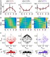
Convexity–concavity tuning in three visual areas. a, Examples of convexity-concavity tuning of three different sites in V1 (left), V4 (center), and PIT (right) measured at each site's preferred orientation and size. Each point on the black curve shows the mean response and SE. Red lines show the polynomial fit. All values are baseline subtracted. b, Tuning fits for sites in V1 (left), V4 (center), and PIT (right). Each row shows a different site and each column shows a graded curvature continuum. Sites were ordered by their A_linear value. c, Scatterplot showing each site's A_linear value (abscissa, convexity vs concavity preferences) and A_quad values (ordinate, symmetry value), all presented according to area (colors). d, Marginal percentage distribution of A_linear values.

Figure 6.

Curvature tuning and preferences for faces. a, Images used to test preferences for faces and objects. b, Classification accuracy (minus shuffled-label baseline) within each area using low-CI or high-CI sites (black and white). c, Classification accuracy within each area by low-CI and high-CI sites when classifying faces versus faces or objects versus objects.

Figure 7.

Relationship between orientation tuning and size. a, Orientation tuning for three V1 sites (animal V); each plot shows responses to a straight Gabors at four different sizes (indicated by colors). b, Mean difference in preferred orientation (±SEM) as a function of Gabor size relative to the biggest Gabor size. Each curve shows a different area. c, Mean Gaussian tuning width as a function of stimulus Gabor size. Asterisks show which tuning curves were statistically different from a flat model (p < 0.050, one-way ANOVA).

References

1. Andrews TJ, Watson DM, Rice GE, Hartley T. Low-level properties of natural images predict topographic patterns of neural response in the ventral visual pathway. J Vis. 2015;15:3. doi: 10.1167/15.7.3. - DOI - PMC - PubMed
1. Bell AH, Malecek NJ, Morin EL, Hadj-Bouziane F, Tootell RB, Ungerleider LG. Relationship between functional magnetic resonance imaging-identified regions and neuronal category selectivity. J Neurosci. 2011;31:12229–12240. doi: 10.1523/JNEUROSCI.5865-10.2011. - DOI - PMC - PubMed
1. Born RT. Center-surround interactions in the middle temporal visual area of the owl monkey. J Neurophysiol. 2000;84:2658–2669. - PubMed
1. Cavanaugh JR, Bair W, Movshon JA. Selectivity and spatial distribution of signals from the receptive field surround in macaque V1 neurons. J Neurophysiol. 2002;88:2547–2556. doi: 10.1152/jn.00693.2001. - DOI - PubMed
1. Chen G, Dan Y, Li CY. Stimulation of non-classical receptive field enhances orientation selectivity in the cat. J Physiol. 2005;564:233–243. doi: 10.1113/jphysiol.2004.080051. - DOI - PMC - PubMed
Publication types
LinkOut - more resources