Reconciling fisheries catch and ocean productivity

Abstract

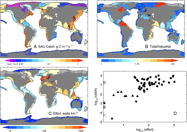
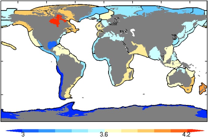
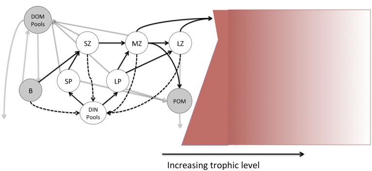
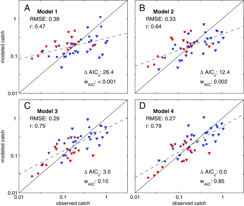
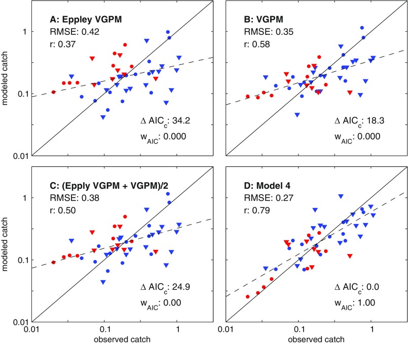
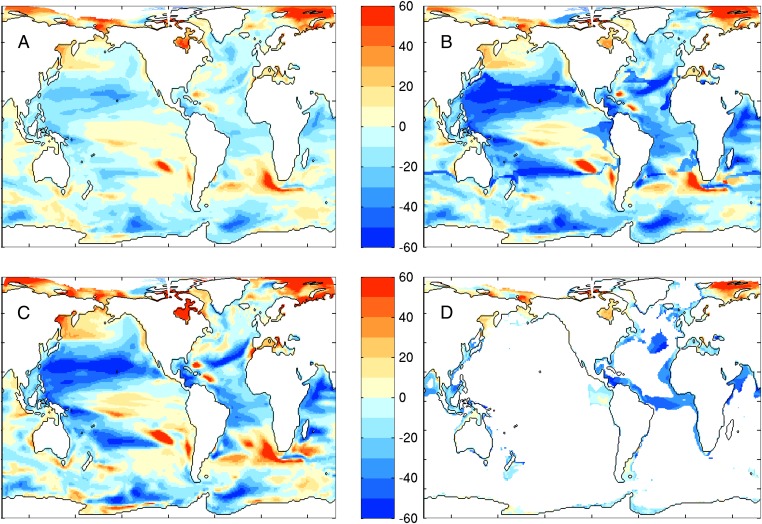
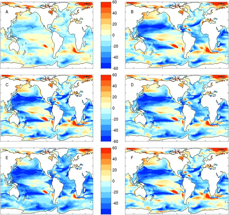
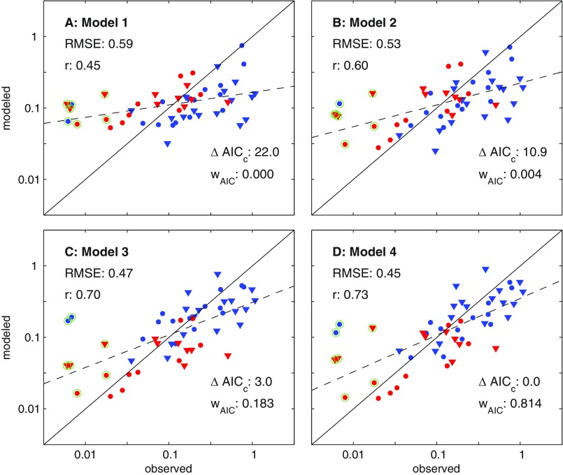
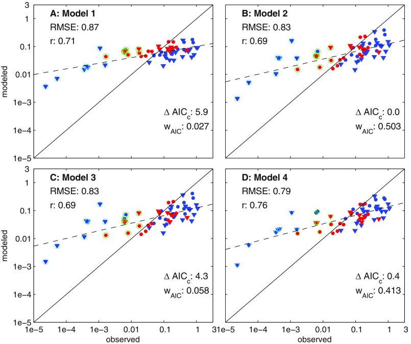
Photosynthesis fuels marine food webs, yet differences in fish catch across globally distributed marine ecosystems far exceed differences in net primary production (NPP). We consider the hypothesis that ecosystem-level variations in pelagic and benthic energy flows from phytoplankton to fish, trophic transfer efficiencies, and fishing effort can quantitatively reconcile this contrast in an energetically consistent manner. To test this hypothesis, we enlist global fish catch data that include previously neglected contributions from small-scale fisheries, a synthesis of global fishing effort, and plankton food web energy flux estimates from a prototype high-resolution global earth system model (ESM). After removing a small number of lightly fished ecosystems, stark interregional differences in fish catch per unit area can be explained (r = 0.79) with an energy-based model that (i) considers dynamic interregional differences in benthic and pelagic energy pathways connecting phytoplankton and fish, (ii) depresses trophic transfer efficiencies in the tropics and, less critically, (iii) associates elevated trophic transfer efficiencies with benthic-predominant systems. Model catch estimates are generally within a factor of 2 of values spanning two orders of magnitude. Climate change projections show that the same macroecological patterns explaining dramatic regional catch differences in the contemporary ocean amplify catch trends, producing changes that may exceed 50% in some regions by the end of the 21st century under high-emissions scenarios. Models failing to resolve these trophodynamic patterns may significantly underestimate regional fisheries catch trends and hinder adaptation to climate change.

Keywords: climate change; fisheries catch; food webs; ocean productivity; primary production.

Fig. 1.

Catch and effort summary. (A) The average of the top 10 annual catches by LME from the SAU catch reconstruction (6) expressed as grams of carbon per square meter per year. A wet weight-to-carbon conversion of 9:1 was used (3). Catch in the central Arctic is very small (<1e-8 g C⋅m⁻²⋅y⁻¹) and is not shown. The black hatching reflects smaller inland seas and embayments not well resolved by ESM2.6 (see text). The gray hatching corresponds to low-effort, low-catch (LELC) outliers from D. (B) The ratio of the average of the top 10 total to top 10 industrial-only catches. The light gray LMEs in the Arctic correspond to systems with no reported industrial catch. (C) The average of the top 10 effort years expressed as integrated effective vessel power (effective watts per square kilometer) (27). The gray LMEs have no effort data but, due to uncertainties in the location of fishing fleets, may have catches (e.g., Chukchi Sea and Aleutian LMEs). (D) Plot of landings in A versus effort in C. The squares are Arctic and Antarctic LMEs, the triangles are Australian LMEs, and the diamond is the insular-Pacific Hawaiian LME. All other points are shown as circles. The open symbols indicate no effort data. These have been placed along the lower effort bound in D, although lack of data does not necessarily imply low effort.

Fig. S1.

The equivalent trophic level of the aggregate catch (TL_eq) calculated via Eq. 4 with trophic efficiency, TE = 0.1.

Fig. S2.

A conceptual diagram of the model for the energy exchanges through the planktonic food web to fish adopted herein (see text for description).

Fig. 2.

Comparison of estimated catches from trophodynamic models 1–4 (A–D) with SAU estimates (6). LMEs are divided in four categories. The red symbols have T₁₀₀ > 20 °C and blue for cooler systems. The triangles correspond to systems where the FDET is larger than MESOZP (i.e., more benthic LMEs), and the circles, to more pelagic LMEs (Fig. S3). ΔAIC_C is the difference in the small-sample Akaike information criterion between the best-fit model (model 4) and each alternative; r, the Pearson correlation; RMSE, root-mean-squared error; w_AIC, Akaike weight, interpreted as the likelihood that this model is closest to the true model (38). The solid line is the 1:1 line, and the dashed line is a linear fit through the model estimated catches.

Fig. S3.

Spatial map of LMEs classified as in Fig. 2. The red points have T₁₀₀ > 20 °C, the blue points have T₁₀₀ < 20 °C, the circles correspond to MESOZP > FDET (more pelagic), and the inverted triangles correspond to MESOZP < FDET (more benthic). We note that classification is sensitive to the offshore extent of LME boundaries, and systems classified as more pelagic may have subregions with energetic benthic food webs. The intent here is only to provide a useful subdivision for interpreting model strengths and weaknesses in the context of this paper. As in the main text, the gray hatching corresponds with LELC outliers. The black hatching corresponds to inland seas and shallow coastal systems that remain poorly resolved by ESM2.6.

Fig. 3.

Energy flow through the planktonic food web. (A) ESM2.6 simulated NPP by LME in grams of carbon per square meter per year. (B) Mesozooplankton production not consumed by other zooplankton (MESOZP) expressed as a fraction of NPP. (C) The flux of detritus to the benthos (FDET) expressed as a fraction of NPP.

Fig. S4.

A–C are fits resulting from using different satellite-based NPP estimates to drive trophodynamic model 1 instead of NPP from ESM2.6. D shows the optimal model 4 fit. All NPP variants are strongly rejected relative to trophodynamic model 4 and (i) show similar underrepresentation of stark cross-LME catch differences, and (ii) strong tendencies to overestimate catch in warm systems and underestimate catch in cold systems.

Fig. 4.

Model 4 parameter uncertainties. (A) Contours of the optimal RMSE for each value of TE_P and TE_B (i.e., the fit reflects an optimization over α, f_T, and T_100,warm for each TE_B, TE_P combination). The gradual slope of the contours across the upper left quadrant of the parameter space and extending into the upper right quadrant indicates weak constraints on TE values across this range. The star corresponds to the best fit in TE_B, TE_P space. The thick black contour corresponds to the 95% confidence interval on TE_B, TE_P. (B) As in A, but the optimal α value for each TE_B, TE_P combination is contoured instead of RMSE. Note the broad range of α values that fall within the 95% TE_B, TE_P confidence intervals and the strong negative correlation between TE values and α.

Fig. 5.

Projected change in NPP and catch under a high-emissions scenario (RCP8.5) from ESM2M-COBALT (25, 69) between 1951–2000 and 2051–2100 using the best-fit trophodynamic model: (A) percent change in NPP, (B) percent change in fish, (C) percent change in MESOZP, and (D) percent change in FDET. FDET changes are only shown for FDET > 2 g C⋅m⁻²⋅y⁻¹ to emphasize changes in systems with significant benthic relative to pelagic fluxes.

Fig. S5.

Comparison of projected percent changes in catch from a range of fish catch models. Differences are between means over the latter half of the 21st century (2051–2100) relative to the latter half of the 20th century (1951–2000). (A) Projected percent change in catch for the best-fit trophodynamic model 1 (i.e., NPP-only model). This model produces much smaller changes in catch but was firmly rejected in favor of alternative models (Fig. 2). (B) Projected catch change for the best-fit trophodynamic model 2. Note the amplification relative to A from accounting for plankton food web dynamics. (C) Projected catch change for the best-fit trophodynamic model 3. (D) Projected catch change for the best fit trophodynamic model 4. (E) Projected change for a “low TE_P” parameter setting (TE_P = 0.05, TE_B = 0.4) that remains statistically indistinguishable from the best case in D. (F) Projected change for a “low TE_B” parameter setting (TE_B = 0.20) that remains statistically indistinguishable from the best case in D. Note the robust nature of amplified catch differences for all trophodynamic models except the strongly rejected trophodynamic model 1.

Fig. S6.

Fits for models 1–4 (A–D) after adding back the Australian and Hawaiian LMEs. Catches in these systems (outlined with green circles) are generally strongly overestimated by the model. This increases the RMSE and decreases the correlation for most models, but the fit still improves significantly with each model iteration and the best solution has the same properties of the fit without these systems: depressed TEs in tropical systems and elevated TEs associated with benthic fluxes (without Australia/Hawaii: α = 0.14, TE_P = 0.14, TE_B = 0.40, f_T = 0.73, T_100,warm = 20 °C; with Australia/Hawaii: α = 0.19, TE_P = 0.10, TE_B = 0.33, f_T = 0.66, T_100,warm = 20 °C).

Fig. S7.

Fits for models 1–4 (A–D), but adding back both the Australian/Hawaiian and Arctic/Antarctic LELC outliers. Australian systems are again circled in green and Arctic systems in light blue. Note the large increase in the range of catches with the introduction of the extremely lightly fished Arctic systems. As described in the main text, all models show high correlation, but this correlation masked large, systematic overestimation of catch in Arctic/Antarctic systems and stark underestimation of most other systems.

Fig. S8.

Comparison of effort versus catch using (A) the mean of the top 10 catch and effort years, calculated independently; and (B) the mean of the top 10 catch years and the mean of the top 10 corresponding effort years. In the latter case, we had to restrict the catch time series to 1950–2006. The LELC clusters are unaffected by these variants in approach. The blue asterisk in A corresponds to the integrated effort/catch values for all regions outside the LMEs. The LELC combination is consistent with these regions accounting for only ∼5% of global catch despite accounting for 78% of ocean area.

References

1. Ryther JH. Photosynthesis and fish production in the sea. Science. 1969;166(3901):72–76. - PubMed
1. Lindeman RL. The trophic-dynamic aspect of ecology. Ecology. 1942;23(4):399–417.
1. Pauly D, Christensen V. Primary production required to sustain global fisheries. Nature. 1995;374(6519):255–257.
1. Libralato S, Pranovi F, Stergiou KI, Link JS. Trophodynamics in marine ecology: 70 years after Lindeman. Mar Ecol Prog Ser. 2014;512:1–7.
1. Coll M, Libralato S, Tudela S, Palomera I, Pranovi F. Ecosystem overfishing in the ocean. PLoS One. 2008;3(12):e3881. - PMC - PubMed
LinkOut - more resources