NEPTUNE'S DYNAMIC ATMOSPHERE FROM KEPLER K2 OBSERVATIONS: IMPLICATIONS FOR BROWN DWARF LIGHT CURVE ANALYSES

Abstract

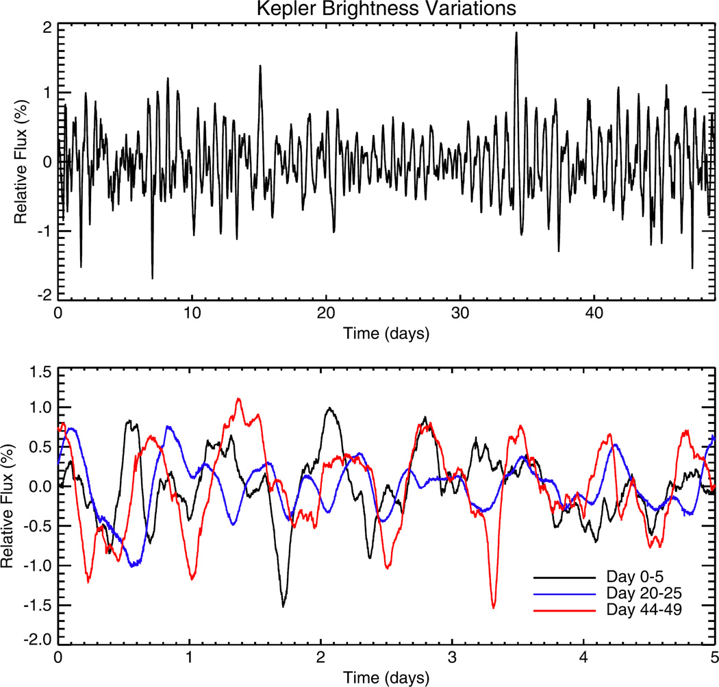
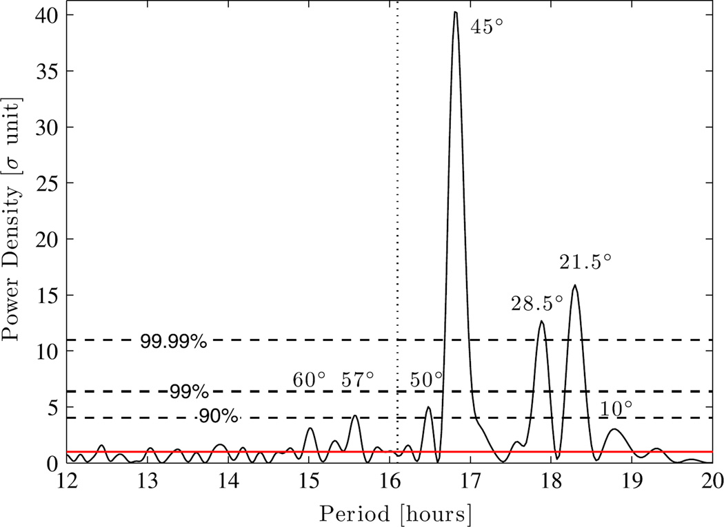
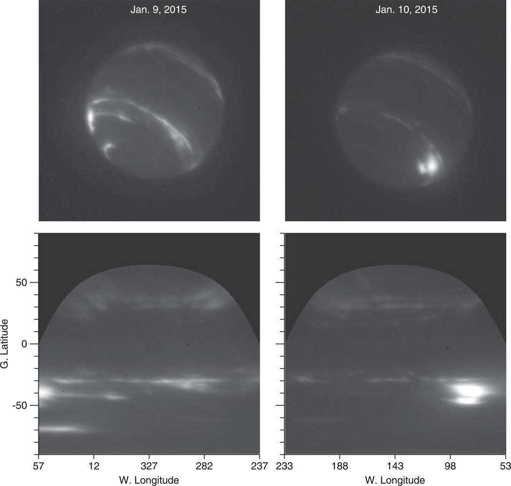
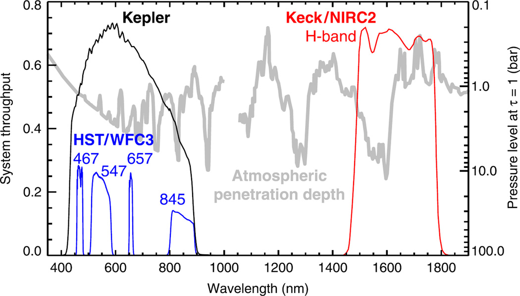
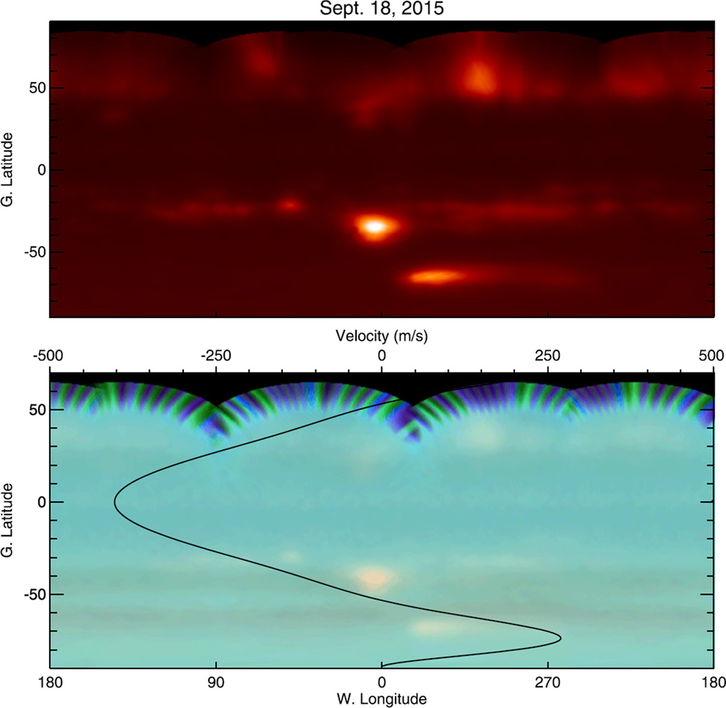
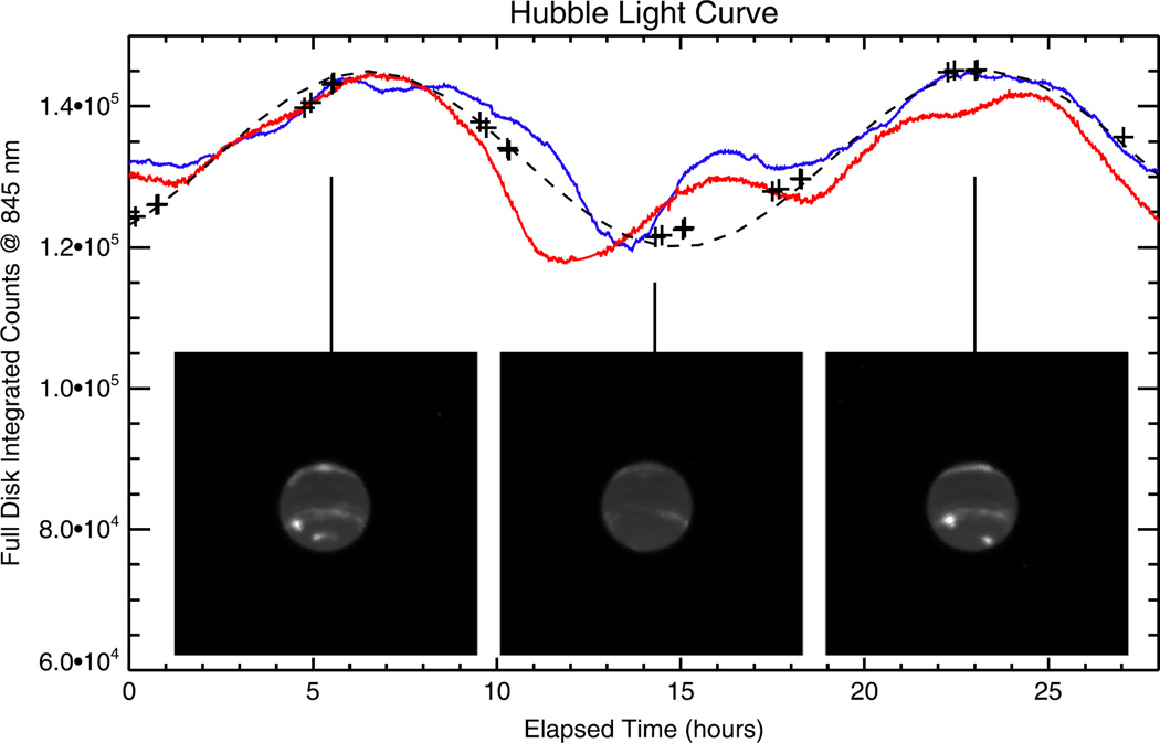
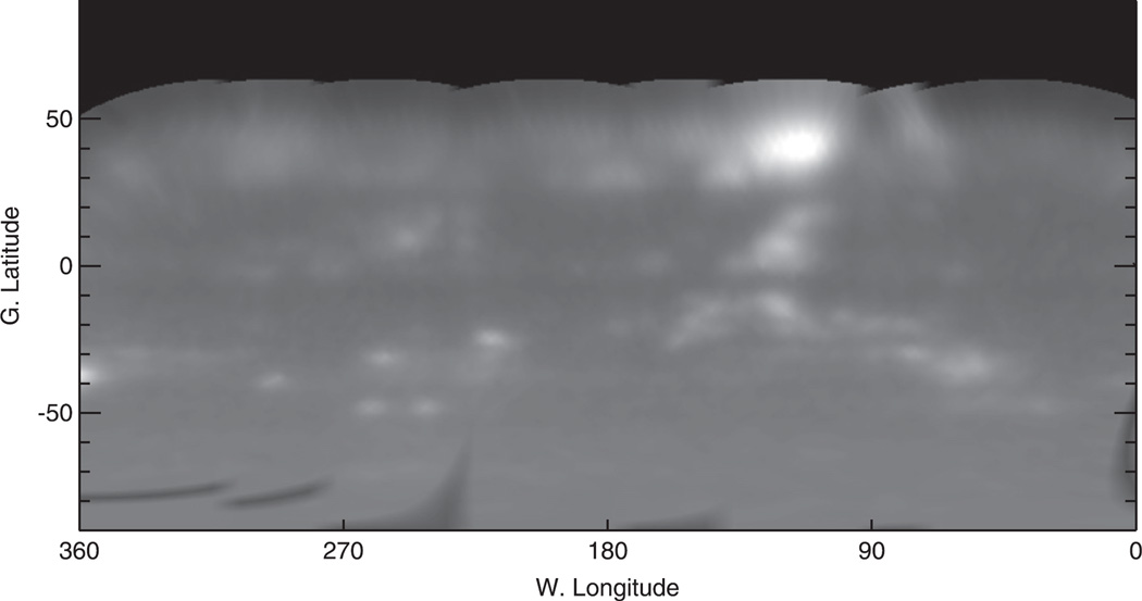
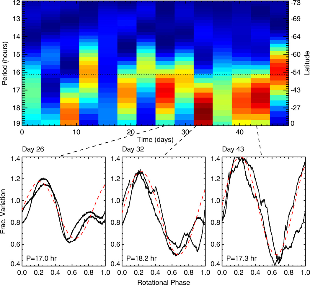
Observations of Neptune with the Kepler Space Telescope yield a 49 day light curve with 98% coverage at a 1 minute cadence. A significant signature in the light curve comes from discrete cloud features. We compare results extracted from the light curve data with contemporaneous disk-resolved imaging of Neptune from the Keck 10-m telescope at 1.65 microns and Hubble Space Telescope visible imaging acquired nine months later. This direct comparison validates the feature latitudes assigned to the K2 light curve periods based on Neptune's zonal wind profile, and confirms observed cloud feature variability. Although Neptune's clouds vary in location and intensity on short and long timescales, a single large discrete storm seen in Keck imaging dominates the K2 and Hubble light curves; smaller or fainter clouds likely contribute to short-term brightness variability. The K2 Neptune light curve, in conjunction with our imaging data, provides context for the interpretation of current and future brown dwarf and extrasolar planet variability measurements. In particular we suggest that the balance between large, relatively stable, atmospheric features and smaller, more transient, clouds controls the character of substellar atmospheric variability. Atmospheres dominated by a few large spots may show inherently greater light curve stability than those which exhibit a greater number of smaller features.

Keywords: brown dwarfs; planets and satellites: atmospheres; planets and satellites: gaseous planets; stars: oscillations (including pulsations); stars: rotation; starspots.

Figure 1

Kepler light curve of Neptune. The top panel shows the full 49 day light curve, with normalized brightness variations over time elapsed since 2014 December 1. The bottom panel shows several 5 day segments emphasizing the evolution of brightness variations with time.

Figure 2

Oversampled and whitened power density spectrum as a function of period. The red line corresponds to the noise level of the whitened spectrum and black dashed lines indicate statistical significance levels. Numbers above some peaks indicate the latitudes on Neptune corresponding to that rotation period based on the zonal velocity curve given by Sánchez-Lavega et al. (2015); the features could be in either hemisphere.

Figure 3

Keck H-band images of Neptune from 2015 January 9 to 10, covering most longitudes. The top panels are unmapped images, and the bottom panels show the latitude and longitude coverage mapped at 2 pixels per degree. These show typical Neptune structure: bright bands of Neptunian cloud activity from planetographic latitude 25° –40° in the northern and southern mid-latitudes, with occasional brighter features.

Figure 4

Spectral sensitivity and atmospheric transmission. Labeled curves show the total spectral sensitivity of Kepler and HST observations (Koch et al. 2010; Dressel 2015). The Keck infrared bandpass includes the NIRC2 H-band filter transmission and detector quantum efficiency, but neglects the telescope optical path outside NIRC2. The atmospheric penetration depth (right axis) is the pressure level where a two-way optical depth of unity is reached in a cloud-free model of Neptune’s atmosphere, including opacity from Rayleigh scattering and gas absorption (from Sromovsky et al. 2001b).

Figure 5

Hubble map of Neptune acquired 2015 September 18. The top panel shows a global map constructed from 845 nm images. The bottom is a visible-wavelength color-composite map (with the blue, green, and red channels mapped to 467, 547, and 657 nm, respectively).We overplot the smoothed zonal wind profile (Sánchez-Lavega et al. 2015), showing winds up to 400 m s⁻¹ (top axis).

Figure 6

Light curve of Neptune from Hubble full-disk brightness at 845 nm (plus signs). A sinusoidal variation, with a 16.8 hr period and arbitrary amplitude, is shown by the dashed line. For comparison, normalized Kepler light curves beginning at Day 6 and Day 25 are shown in blue and red, respectively. (An animation of this figure is available.)

Figure 7

Neptune global map from Hubble WFC3/UVIS acquired 2011 June 25–26 at 845 nm. High northern latitudes were not visible, and a bad column resulted in artifacts at high southern latitudes; no SPF is visible.

Figure 8

Short-interval periodogram analysis. The top panel shows the Lomb-Scargle periodogram in 3.5 day segments; red indicates higher spectral power. The remaining panels show the Kepler brightness variations (black curves) from three of the segments, rotationally phased to the corresponding period of maximum spectral power from the periodogram, and plotted over two rotations within that interval; the most significant period is shown as a dashed red line for each date.

Figure 9

Fourier transform of the Kepler light curve. Gray line is the power density spectrum of the Kepler light curve in parts per million (ppm) per µHz, as function of frequency (µHz). The blue peaks match Neptune’s rotation frequency and two harmonics. The black line is the power density smoothed over 100 bins to guide the eye to the mean noise level. The plain green line indicates the noise model, which is the sum of two semi-Lorentzians and a white noise offset (dashed red lines).

References

1. Apai D, Radigan J, Buenzil E, et al. ApJ. 2013;768:121.
1. Appourchaux T, Berthomieu G, Michel E, et al. In: ESA Special Publication 1306, Data Analysis Tools for the Seismology Programme. Fridlund M, et al., editors. Noordwijk: ESA; 2006. p. 377.
1. Artigau E, Bouchard S, Doyon R, Lafreniere D. ApJ. 2009;701:1534.
1. Bailer-Jones CAL, Mundt R. A&A. 2001;367:218.
1. Batalha NM. PNAS. 2014;111:12647. - PMC - PubMed
LinkOut - more resources