

Spectral Methods for Numerical Relativity
- PMID: 28163610
- PMCID: PMC5253976
- DOI: 10.12942/lrr-2009-1
Spectral Methods for Numerical Relativity
Abstract
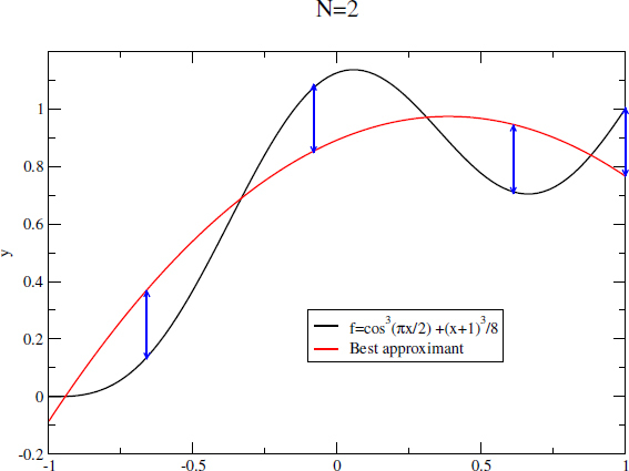
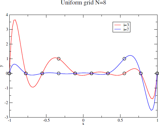
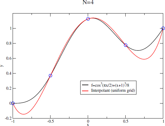
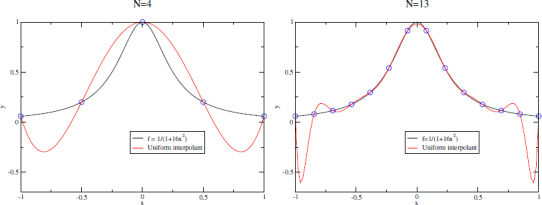
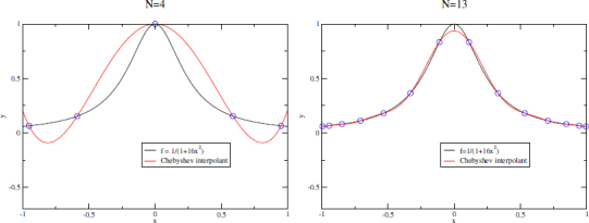
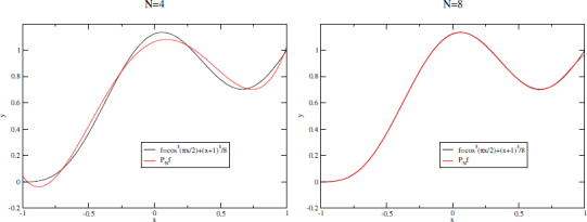
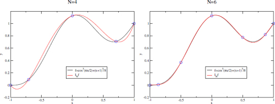
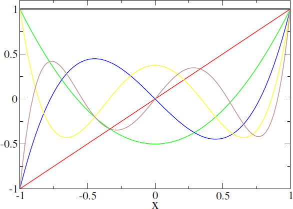
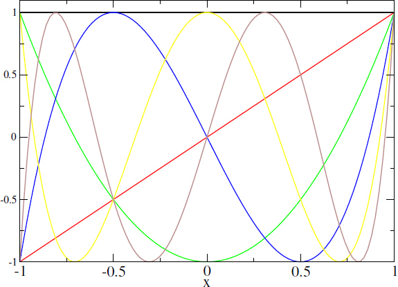
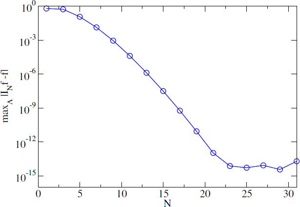
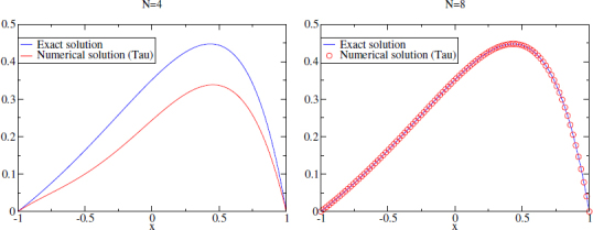
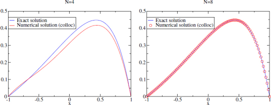
Equations arising in general relativity are usually too complicated to be solved analytically and one must rely on numerical methods to solve sets of coupled partial differential equations. Among the possible choices, this paper focuses on a class called spectral methods in which, typically, the various functions are expanded in sets of orthogonal polynomials or functions. First, a theoretical introduction of spectral expansion is given with a particular emphasis on the fast convergence of the spectral approximation. We then present different approaches to solving partial differential equations, first limiting ourselves to the one-dimensional case, with one or more domains. Generalization to more dimensions is then discussed. In particular, the case of time evolutions is carefully studied and the stability of such evolutions investigated. We then present results obtained by various groups in the field of general relativity by means of spectral methods. Work, which does not involve explicit time-evolutions, is discussed, going from rapidly-rotating strange stars to the computation of black-hole-binary initial data. Finally, the evolution of various systems of astrophysical interest are presented, from supernovae core collapse to black-hole-binary mergers.
Figures


Similar articles
-
Numerical relativity of compact binaries in the 21st century.Rep Prog Phys. 2019 Jan;82(1):016902. doi: 10.1088/1361-6633/aadb16. Epub 2018 Aug 17. Rep Prog Phys. 2019. PMID: 30117809
-
Numerical Hydrodynamics in General Relativity.Living Rev Relativ. 2003;6(1):4. doi: 10.12942/lrr-2003-4. Epub 2003 Aug 19. Living Rev Relativ. 2003. PMID: 29104452 Free PMC article. Review.
-
Numerical Hydrodynamics and Magnetohydrodynamics in General Relativity.Living Rev Relativ. 2008;11(1):7. doi: 10.12942/lrr-2008-7. Epub 2008 Sep 19. Living Rev Relativ. 2008. PMID: 28179823 Free PMC article. Review.
-
Continuum and Discrete Initial-Boundary Value Problems and Einstein's Field Equations.Living Rev Relativ. 2012;15(1):9. doi: 10.12942/lrr-2012-9. Epub 2012 Aug 27. Living Rev Relativ. 2012. PMID: 28179838 Free PMC article. Review.
-
Collapse of magnetized hypermassive neutron stars in general relativity.Phys Rev Lett. 2006 Jan 27;96(3):031101. doi: 10.1103/PhysRevLett.96.031101. Epub 2006 Jan 25. Phys Rev Lett. 2006. PMID: 16486677
Cited by
-
Rotating stars in relativity.Living Rev Relativ. 2017;20(1):7. doi: 10.1007/s41114-017-0008-x. Epub 2017 Nov 29. Living Rev Relativ. 2017. PMID: 29225510 Free PMC article. Review.
-
Exploring New Physics Frontiers Through Numerical Relativity.Living Rev Relativ. 2015;18(1):1. doi: 10.1007/lrr-2015-1. Epub 2015 Sep 21. Living Rev Relativ. 2015. PMID: 28179851 Free PMC article. Review.
-
Grid-based Methods in Relativistic Hydrodynamics and Magnetohydrodynamics.Living Rev Comput Astrophys. 2015;1(1):3. doi: 10.1007/lrca-2015-3. Epub 2015 Dec 22. Living Rev Comput Astrophys. 2015. PMID: 30652121 Free PMC article. Review.
-
Companion-based multi-level finite element method for computing multiple solutions of nonlinear differential equations.Comput Math Appl. 2024 Aug 15;168:162-173. doi: 10.1016/j.camwa.2024.05.035. Epub 2024 Jun 14. Comput Math Appl. 2024. PMID: 39726586 Free PMC article.
-
Coalescence of Black Hole-Neutron Star Binaries.Living Rev Relativ. 2011;14(1):6. doi: 10.12942/lrr-2011-6. Epub 2011 Aug 29. Living Rev Relativ. 2011. PMID: 28163619 Free PMC article. Review.
References
-
- Alcubierre M, Brandt S, Brügmann B, Gundlach C, Massó J, Seidel E, Walker P. Test-beds and applications for apparent horizon finders in numerical relativity. Class. Quantum Grav. 2000;17:2159–2190. doi: 10.1088/0264-9381/17/11/301. - DOI
-
- Alcubierre M, et al. Towards standard testbeds for numerical relativity. Class. Quantum Grav. 2004;21:589–613. doi: 10.1088/0264-9381/21/2/019. - DOI
-
- Amsterdamski P, Bulik T, Gondek-Rosińska D, Kluźniak W. Marginally stable orbits around Maclaurin spheroids and low-mass quark stars. Astron. Astrophys. 2002;381:L21–L24. doi: 10.1051/0004-6361:20011555. - DOI
Publication types
LinkOut - more resources
Full Text Sources