Gravitational Waves from Gravitational Collapse

Abstract

Gravitational-wave emission from stellar collapse has been studied for nearly four decades. Current state-of-the-art numerical investigations of collapse include those that use progenitors with more realistic angular momentum profiles, properly treat microphysics issues, account for general relativity, and examine non-axisymmetric effects in three dimensions. Such simulations predict that gravitational waves from various phenomena associated with gravitational collapse could be detectable with ground-based and space-based interferometric observatories. This review covers the entire range of stellar collapse sources of gravitational waves: from the accretion-induced collapse of a white dwarf through the collapse down to neutron stars or black holes of massive stars to the collapse of supermassive stars.

Electronic supplementary material: Supplementary material is available for this article at 10.12942/lrr-2011-1.

Figure 1

Diagram of the convective engine for supernova explosions.

Figure 2

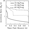
Accretion rates of different mass stars. The more massive stars have higher accretion rates and are, hence, harder to explode. Figure 1 from Fryer [97].

Figure 3

Supernova explosion energies (dotted lines) based on simulation (solid circles) and observation (solid dot of SN 1987A) as a function of progenitor mass. The binding energy of the envelop (material beyond the 3 M_⊙ core) rises dramatically at 20 M_⊙ (solid line). This fast rise with mass and the decline based on explosion simulations of the energies from the convective engine mean that even if the errors in these estimates are large, the likely dividing line between neutron star and black hole formation can be determined fairly accurately. Figure 1 of Fryer & Kalogera [109].

Figure 4

Fate of massive stars as a function of mass and metallicity. Figure 1 from Heger et al. [136].

Figure 5

Explosion energy as a function of launch time of the supernova shock for four differently-massed stars assuming the energy is stored in the convective region. The energy is then limited by the ram pressure of the infalling stellar material. Note that it is difficult to make a strong explosion after a long delay. For more details, see [99] and Fryer et al. (in preparation).

Figure 6

Left-hand panel: Evolution of the core-collapse supernova rate with redshift. The dashed line shows the intrinsic total supernova rate derived from the star formation density. The supernova rate that can be recovered by optical searches is shown in light gray, and is compared with the data points from Cappellaro et al. [44] (squares) and Dahlen et al. [59] (circles). Right-hand panel: Fraction of CC SNe that are not present in the optical and near-IR searches as a function of redshift. (Figure 2 of Mannucci et al. [193]; used with permission.)

Figure 7

Six snapshots in time of the convection in the collapse of a 23 M_⊙ star. The plot displays slices of the data in the x-z plane. The vectors denote direction and magnitude of the particle motion. The colors denote entropy. The convection is far from symmetric, but we do not get the single-sided downflows seen in many recent 2-dimensional calculations. Figure 4 of [116].

Figure 8

Images of the gas entropy (red is higher than the equilibrium value, blue is lower) illustrate the instability of a spherical standing accretion shock. This model has γ = 4/3 and is perturbed by placing overdense rings into the infalling preshock gas. The shock is kept stalled by using a cooling function. Note that with the scaling for a realistic supernova model, the last image on the right corresponds to 300 ms. These simulations are axisymmetric, forcing a reflection symmetry about the vertical axis. (Figure 6 of [21]; used with permission.)

Figure 9

Mean angular momenta vs. mass for both merged stars just after the merger and at collapse. The thick solid line at the top of the graph is the angular momentum just after merger. Dotted lines correspond to different mappings of the 3-dimensional merger calculation into the 1-dimensional stellar evolution code. We also plotted the angular momentum for material at the innermost stable circular orbit for a non-rotating black hole vs. mass (thin solid line). Figure 5 of [104].

Figure 10

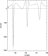
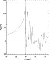
Type I waveform (quadrupole amplitude as a function of time) from one of Zwerger and Müller’s [350] simulations of a collapsing polytrope. The vertical dotted line marks the time at which the first bounce occurred. (Figure 5d of [350]; used with permission.)

Figure 11

Type II waveform (quadrupole amplitude as a function of time) from one of Zwerger and Müller’s [350] simulations of a collapsing polytrope. The vertical dotted line marks the time at which bounce occurred. (Figure 5a of [350]; used with permission.)

Figure 12

Type III waveform (quadrupole amplitude as a function of time) from one of Zwerger and Müller’s [350] simulations of a collapsing polytrope. The vertical dotted line marks the time at which bounce occurred. (Figure 5e of [350]; used with permission).

Figure 13

mpeg-Movie (11.2 MB) Still from a movie showing The evolution of the regular collapse model A3B2G4 of Dimmelmeier et al. [67]. The left frame contains the 2D evolution of the logarithmic density. The upper and lower right frames display the evolutions of the gravitational wave amplitude and the maximum density, respectively. (For video see appendix)

Figure 14

mpeg-Movie (10.0 MB) Still from a movie showing Same as Movie 13, but for rapid collapse model A3B2G5 of Dimmelmeier et al. [67]. (For video see appendix)

Figure 15

mpeg-Movie (11.8 MB) Still from a movie showing Same as Movie 13, but for multiple collapse model A2B4G1 of Dimmelmeier et al. [67]. (For video see appendix)

Figure 16

mpeg-Movie (8.51 MB) Still from a movie showing Same as Movie 13, but for rapid, differentially-rotating collapse model A4B5G5 of Dimmelmeier et al. [67]. (For video see appendix)

Figure 17

The gravitational waveform (including separate matter and neutrino contributions) from the collapse simulations of Burrows and Hayes [37]. The curves plot the GW amplitude of the source as a function of time. (Figure 3 of [37]; used with permission.)

Figure 18

The gravitational waveform for matter contributions from the asymmetric collapse simulations of Fryer et al. [107]. The curves plot the GW amplitude of the source as a function of time. (Figure 3 of [107]; used with permission.)

Figure 19

Convective instabilities inside the proto neutron star in the 2D simulation of Müller and Janka [208]. The evolutions of the temperature (left panels) and logarithmic density (right panels) distributions are shown for the radial region 15–95 km. The upper and lower panels correspond to times 12 and 21 ms, respectively, after the start of the simulation. The temperature values range from 2.5 × 10¹⁰ to 1.8 × 10¹¹ K. The values of the logarithm of the density range from 10.5 to 13.3 g cm⁻³. The temperature and density both increase as the colors change from blue to green, yellow, and red. (Figure 7 of [208]; used with permission.)

Figure 20

Quadrupole amplitudes [cm] from convective instabilities in various models of [208]. The upper left panel is the amplitude from a 2D simulation of proto neutron star convection. The other three panels are amplitudes from 2D simulations of hot bubble convection. The imposed neutrino flux in the hot bubble simulations increases from the top right model through the bottom right model. (Figure 18 of [208]; used with permission.)

Figure 21

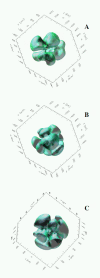
gif-Movie (15.6 MB) Still from a movie showing Isosurface of material with radial velocities of 1000 km s⁻¹ for three different simulation resolutions. The isosurface outlines the outward moving convective bubbles. The open spaces mark the downflows. Note that the upwelling bubbles are large and have very similar size scales to the two-dimensional simulations. From Fryer & Warren [112]. (For video see appendix)

Figure 22

avi-Movie (3.98 MB) Still from a movie showing The oscillation of the proto neutron star caused by downstreams in the SASI-induced convective region above the proto neutron star. From Burrows et al. [40]. (For video see appendix)

Figure 23

A comparison between the GW amplitude h(f) for various sources and the LIGO-II sensitivity curve based on the analytic estimates from FHH [106]. See the text for details regarding the computations of h. The SNe sources at 10 Mpc; and the Population III sources at a luminosity distance of ∼ 50 Gpc. Secular bar-mode sources are identified with an (s), dynamical bar modes with a (d). This assumes strong bar modes exist, which has not been demonstrated robustly.

Figure 24

mov-Movie (9.34 MB) Still from a movie showing Evolution of a secular bar instability, see Ou et al. [236] for details. (For video see appendix)

Figure 25

β and instability growth time versus mass in the proto black hole formed in the collapse of a 300 M_⊙ star at bounce (dotted line) and just prior to black-hole formation (solid line). Figure 10 of [115].

Figure 26

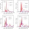
The GW signal from convection in a proto neutron star. The top panel shows the GW quadrupole amplitude as a function of time for both the convective mass flow (thick line) and anisotropic neutrino emission (thin line). The combined spectral energy distribution of the quadrupole radiation for both sources is shown in the middle figure, with just the neutrino component alone in the bottom panel. Note that although the quadrupole amplitude for the neutrino emission is much higher, it varies slower than the mass motions. Hence, it only dominates the signal at low frequencies. (Figures from [209]; used with permission.)

Figure 27

Detection limits of TAMA, first LIGO, advanced LIGO, and Large-scale Cryogenic Gravitational wave Telescope (LCGT) with the expected GW spectrum obtained from the numerical simulations. The left panel shows the GW spectrum contributed from neutrinos (solid) and from the matter (dashed) in a rotating model with Ω = 4 rad s⁻¹ imposed initially on a 15 M_⊙ progenitor model. In the right panel, the open circles and the pluses represent the amplitudes of h_ν,eq with the characteristic frequencies of ν_eq for the models with the cylindrical and the shell-type rotation profiles, respectively. Under the frequency of ν_eq, the GWs from the neutrinos dominate over those from the matter contributions. From the panel, it is seen that the GWs from neutrinos dominate over the ones from the matter in a lower frequency (f ≤ 100 Hz). Note that the source is assumed to be located at the distance of 10 kpc. (Figures from [166]; used with permission.)

Figure 28

The gravitational waveform for neutrino contributions from the asymmetric collapse simulations of Fryer et al. [107]. The curves plot the product of the GW amplitude to the source as a function of time. (Figures from [107]; used with permission.)

Figure 29

The matter density in the equatorial plane of the rapidly-rotating collapsar simulation, 0.44 s after collapse. The spiral wave forms near the center of the collapsar 0.29 s after collapse and moves outward through the star. (Figure 4 of [250]; used with permission.)

Figure 30

A comparison between the GW amplitude h(f) for various sources and the LISA noise curve. See the text for details regarding the computations of h. The SMS sources are assumed to have masses of ∼ 10⁶ M_⊙ and be located at a luminosity distance of 50 Gpc. The bar-mode source is a dynamical bar mode.

Figure 31

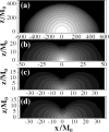
Meridional plane density contours from the SMS collapse simulation of Saijo, Baumgarte, Shapiro, and Shibata [259]. The contour lines denote densities ρ = ρ_c × d^{(1 − i/16)}, where ρ_c is the central density. The frames are plotted at (t/t_D, ρ_c, d) = (a) (5.0628 × 10⁻⁴, 8.254 × 10⁻⁹, 10⁻⁷), (b) (2.50259, 1.225 × 10⁻⁴, 10⁻⁵), (c) (2.05360, 8.328 × 10⁻³, 5.585 × 10⁻⁷), (d) (2.50405, 3.425 × 10⁻², 1.357 × 10⁻⁷). Here t, t_D, and M₀ are the time, dynamical time , where R_e is the initial equatorial radius and M is the mass), and rest mass. (Figure 15 of [259]; used with permission.)

Figure 32

GW signals from matter motions in the bounce and convection phases of stellar collapse. These limits and estimates have not changed from the previous publication of this Living Reviews article [111]. Uncertainties in the estimates still allow variations within an order of magnitude of these results. The LIGO and advanced LIGO sensitivities are included for reference. The limits are not upper limits of a single signal, but upper limits of all possible signals (varying the conditions of the collapse). This figure does not represent a single signal.

Figure 33

GW signals from asymmetric neutrino emission in the bounce and convection phases of stellar collapse. These limits and estimates have not changed from the previous publication of this Living Reviews article [111]. Uncertainties in the estimates still allow variations within an order of magnitude of these results. The LIGO and advanced LIGO sensitivities are included for reference. The limits are not upper limits of a single signal, but upper limits of all possible signals (varying the conditions of the collapse). This figure does not represent a single signal.

References

1. Abel T, Bryan GL, Norman ML. The Formation and Fragmentation of Primordial Molecular Clouds. Astrophys. J. 2000;540:39–44. doi: 10.1086/309295. - DOI
1. Akiyama S, Wheeler JC. Magnetic Fields in Supernovae. In: Fryer CL, editor. Stellar Collapse; Dordrecht; Boston: Kluwer Academic Publishers; 2004. pp. 259–275.
1. Akiyama S, Wheeler JC, Meier DL, Lichtenstadt I. The Magnetorotational Instability in Core-Collapse Supernova Explosions. Astrophys. J. 2003;584:954–970. doi: 10.1086/344135. - DOI
1. Andersson N. A New Class of Unstable Modes of Rotating Relativistic Stars. Astrophys. J. 1998;502:708–713. doi: 10.1086/305919. - DOI
1. Andersson N. Gravitational waves from instabilities in relativistic stars. Class. Quantum Grav. 2003;20:R105–R144. doi: 10.1088/0264-9381/20/7/201. - DOI
LinkOut - more resources