

Review
doi: 10.12942/lrr-2011-6.
Epub 2011 Aug 29.
Coalescence of Black Hole-Neutron Star Binaries
Affiliations
- PMID: 28163619
- PMCID: PMC5255529
- DOI: 10.12942/lrr-2011-6
Item in Clipboard
Review
Coalescence of Black Hole-Neutron Star Binaries
Living Rev Relativ.
2011.
Abstract
We review the current status of general relativistic studies for the coalescence of black hole-neutron star (BH-NS) binaries. First, procedures for a solution of BH-NS binaries in quasi-equilibrium circular orbits and the numerical results, such as quasi-equilibrium sequence and mass-shedding limit, of the high-precision computation, are summarized. Then, the current status of numerical-relativity simulations for the merger of BH-NS binaries is described. We summarize our understanding for the merger and/or tidal disruption processes, the criterion for tidal disruption, the properties of the remnant formed after the tidal disruption, gravitational waveform, and gravitational-wave spectrum.
Figures
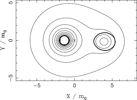
Contours of the conformal factor ψ in the equatorial plane for the innermost configuration with Q = 3 and  shown in [210]. The cross “×” indicates the position of the rotation axis.
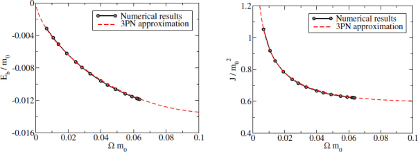
Binding energy Eb/m0 (left panel) and total angular momentum  (right panel) as functions of Ωm0 for binaries of mass ratio Q = 3 and NS mass
  [210]. The solid curve with filled circles show numerical results, and the dashed curve denotes the results in the 3PN approximation [25].
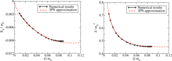
The same as Figure 2 but for the sequence of mass ratio Q = 5 [210].
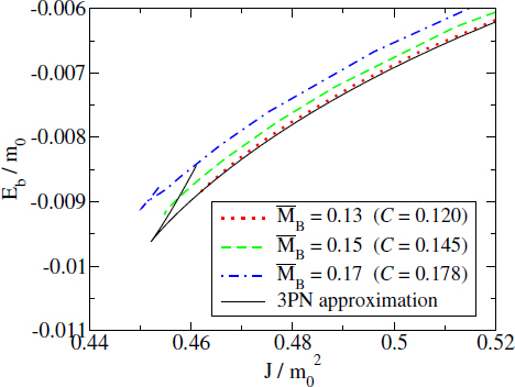
The binding energy as a function of total angular momentum for binaries of mass ratio Q = 5, and different NS compactness [210]. The solid curve denotes the results in the 3PN approximation [25].
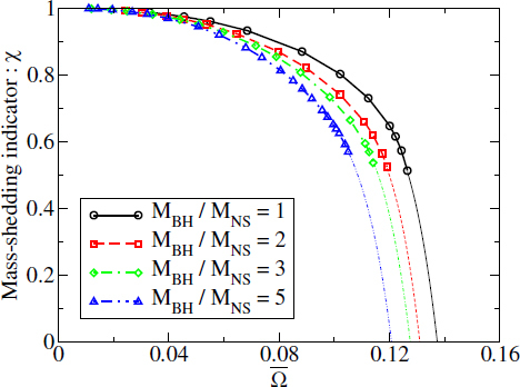
Extrapolation of sequences for NS compactness  to the mass-shedding limit (χ = 0). The thick curves are sequences constructed using numerical data, and the thin curves are extrapolated sequences [210]. Note that the horizontal axis is the orbital angular velocity in polytropic units,
  .
.
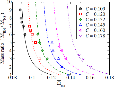
Fits of the mass-shedding limit by the analytic expression (101) [210]. The mass-shedding limit for each NS compactness and mass ratio is computed by the extrapolation of the numerical data.
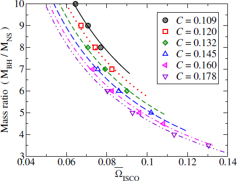
Fits of the minimum point of the binding energy curve by expression (103) [210].
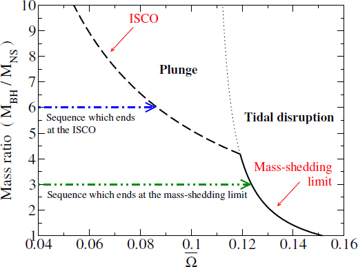
An example of the boundary between the mass-shedding limit and the ISCO [210]. The selected model is the case of  . The solid curve denotes the mass-shedding limit, and the long-dashed one the ISCO for each mass ratio as a function of the orbital angular velocity in polytropic units. The dotted curve denotes the mass-shedding limit for unstable quasi-equilibrium sequences.
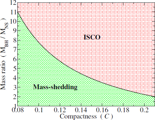
Critical mass ratio, which separates BH-NS binaries that encounter an ISCO before reaching mass shedding and undergoing tidal disruption, as a function of the compactness of NS. This figure is drawn for the model of Γ = 2 polytropic EOS [210].
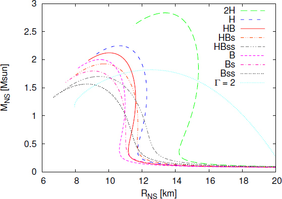
The relation between the mass and the circumferential radius of a spherical NS with piecewise polytropic EOS for which parameters are described in Table 4. For comparison, the curve for the Γ = 2 polytropic EOS with κ/c2 = 2 × 10⁻¹⁶ in cgs units is also plotted (dotted curve). The figure is taken from [107]. Note that if the observational result of [51] (if the presence of an ≈ 1.97 M⊙ NS) is confirmed by 100%, some of the soft EOS displayed here will be ruled out.
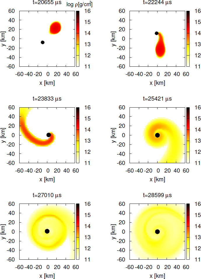
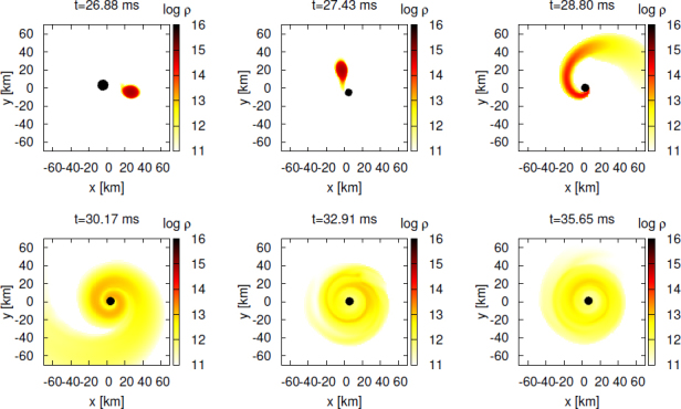
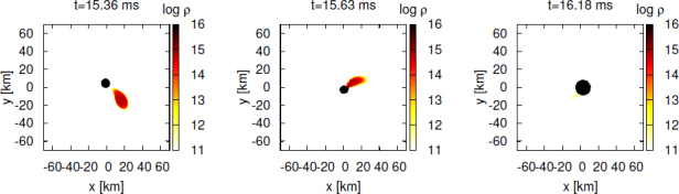
Evolution of the rest-mass density profile in units of g/cm3 and the location of the apparent horizon on the equatorial plane for a model with MBH = 2.7 M⊙, a = 0, MNS = 1.35 M⊙, and RNS = 15.2 km (EOS 2H). This simulation was performed by the KT group. The filled circle denotes the region inside the apparent horizon of the BH. The colored panel on the right-hand side of each figure shows log10(ρ). This figure is taken from [107].
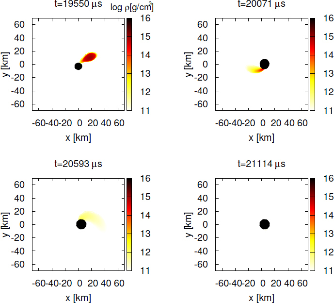
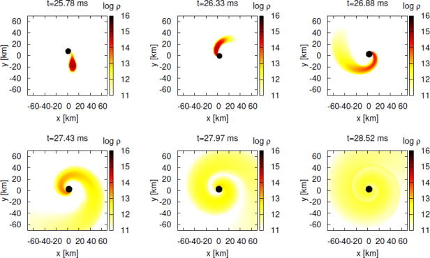
The same as Figure 11 but for a model with MBH = 4.05 M⊙, a = 0, MNS = 1.35 M⊙, and RNS = 11.0 km (EOS B).
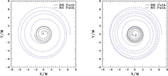
Trajectories of the BH and NS coordinate centroids for models with Q = 3,  , and a = 0 (left) and a = 0.75 (right). This simulation was performed by the UIUC group. The NS is modeled by the Γ-law EOS with Γ = 2. The BH coordinate centroid corresponds to the centroid of the BH, and the NS coordinate centroid denotes a mass center. This figure is taken from [63].
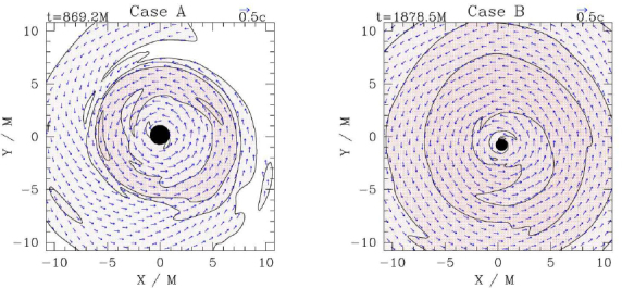
A remnant BH-disk system for models shown in Figure 13. The simulation was performed by the UIUC group. The contour curves, velocity fields (arrows), and BH (solid circles) are plotted. This figure is taken from [63].
The same as Figure 11 but for a model with MBH = 4.05 M⊙, a = 0.75, MNS = 1.35 M⊙, and RNS = 11.6 km (EOS HB). The simulation was performed by the KT group. The figure is taken from [109].
The same as Figure 15 but for a model with a = 0.5. This simulation was performed by the KT group. This figure is taken from [109].
The same as Figure 16 but for a model with a = −0.5. This simulation was performed by the KT group. This figure is taken from [109].
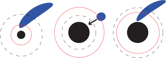
Schematic pictures for the three types of merger process that have been found to date. Left (type-I): the NS is tidally-disrupted and the extent of the tidally disrupted material is as large as or larger than the BH surface area. Middle (type-II): the NS is not tidally disrupted and simply swallowed by the BH. Right (type-III): the NS is tidally disrupted and the extent of the tidally disrupted material in the vicinity of the BH horizon is smaller than the BH surface area. The solid black sphere is the BH, the blue distorted ellipsoid is the NS, the solid red circle is the location of the BH ISCO, and the dashed circle is the location of the tidal-disruption limit. This figure is taken from [109].
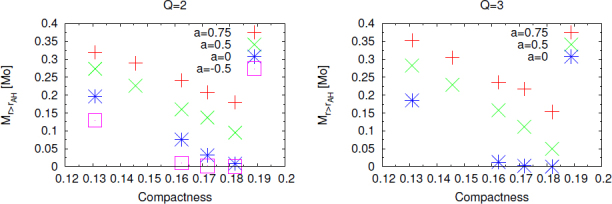
Left: Disk mass at 10 ms after the onset of merger as a function of NS compactness  with various piecewise polytropic EOS and with various values of a for Q = 2. Right: The same as the left panel but for Q = 3. The simulations were performed by the KT group and the figure is taken from [109].
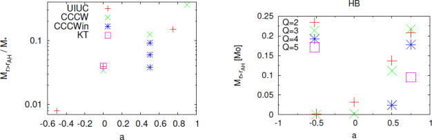
Left: Summary of the remnant disk mass as a function of the BH spin for a fixed EOS (Γ = 2 EOS), NS compactness  , and mass ratio (Q = 3), computed by the UIUC, CCCW, and KT groups. The vertical axis shows the fraction of the disk mass Mr>rAH/MB where MB is the baryon rest mass of the NS. “CCCWin” shows the results by the CCCW group with inclination angle of the BH spin, 40, 60, and 80 degrees (from upper to lower points). Right: The same as the left panel but for the disk mass in the solar mass unit for more compact NS
  with a piecewise polytropic EOS (HB). The simulation was performed by the KT group [109]. For both panels, the disk mass is measured at t ≈ 10 ms after the onset of the merger (for the Γ-law EOS, MNS is assumed to be 1.4 M∩).
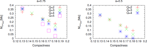
Left: Disk mass as a function of NS compactness for various values of Q with a = 0.75. Right: The same as the left panel but for a = 0.5. These simulations were performed by the KT group and this figure is taken from [109].
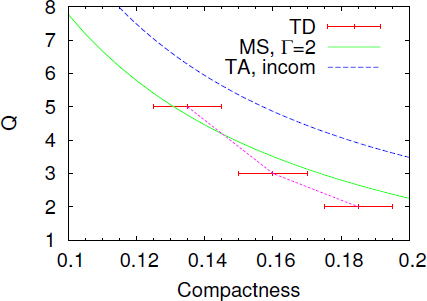
A summary for the conditions of tidal disruption and mass shedding for a = 0 in the plane of  . If the value of Q or
  is smaller than that of the threshold curves shown here, they occur. The points with error bars (and the dotted curve) approximately denote the numerical results for tidal disruption, based on results by the KT group for Q = 2, by the CCCW, KT, and UIUC groups for Q = 3, and by the AEI group for Q = 5. The solid and dashed curves denote the critical curves for the onset of mass shedding for Γ = 2 EOS in general relativity [209, 210], and for the incompressible fluid in a tidal approximation (see Equation (12)), respectively.
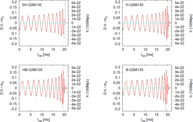
Gravitational waveforms observed along the axis perpendicular to the orbital plane for Q = 3 and a = 0 with very stiff (2H), stiff (H), moderate (HB), and soft (B) EOS. The simulation was performed by the KT group. The solid and dashed curves denote the numerical results and results derived by the Taylor-T4 formula. D is the distance from the source and m0 = MBH + MNS. The left and right axes show the normalized amplitude (c2Dh/Gm0) and physical amplitude for D = 100 Mpc, respectively. This figure is taken from [107].
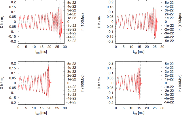
The same as Figure 23 but for Q = 3 and a = 0.75 (top left), 0.5 (top right), 0 (bottom left), and −0.5 (bottom right) with HB EOS. This figure is taken from [109].
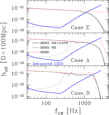
The gravitational-wave spectrum for Q = 1 (Case E), 3 (Case A), and 5 (Case D) with a = 0 and Γ-law EOS with Γ = 2. This simulation was performed by the UIUC group. The solid curve shows the spectrum of a 2.5PN and numerical waveforms, while the dotted curve shows the contribution from the numerical waveform only. The dashed curve is the analytic fit derived in [5] from analysis of BH-BH binaries composed of a non-spinning BH with the same values of Q as the BH-NS. The heavy solid curve is the effective strain of Advanced LIGO. To set physical units, a rest mass is assumed to be MB = 1.4 M⊙ (R ≈ 13 km) for the NS and a source distance of D = 100 Mpc. This figure is taken from [63].
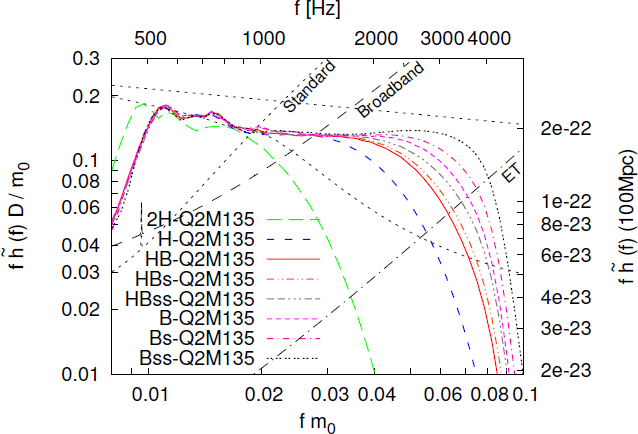
Spectra of gravitational waves from BH-NS binaries for Q = 2, a = 0, and MNS = 1.35 M⊙ with various EOS. The bottom axis denotes the normalized dimensionless frequency fm0(= Gfm0/c3) and the left axis the normalized amplitude c2
 . The top axis denotes the physical frequency f in Hz and the right axis the effective amplitude
  observed at a distance of 100 Mpc from the binaries. The short-dashed sloped line plotted in the upper left region denotes a planned noise curve of Advanced-LIGO [2] optimized for 1.4 M⊙ NS-NS inspiral detection (“Standard”), the long-dashed slope line denotes a noise curve optimized for burst detection (“Broadband”) and the dot-dashed slope line plotted in the lower right region denotes a planned noise curve of the Einstein Telescope (“ET”) [91, 92]. The upper transverse dashed line is the spectrum derived by the quadrupole formula and the lower one is the spectrum derived by the Taylor-T4 formula, respectively. This figure is taken from [107].
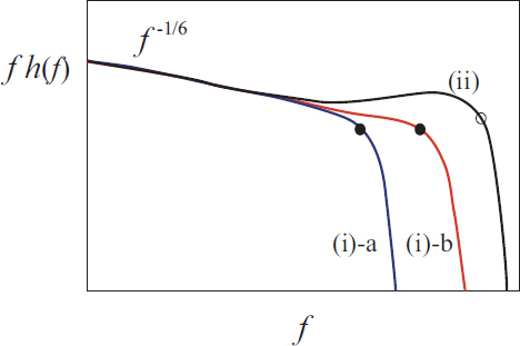
Schematic figure for the gravitational-wave spectrum for the same masses of BH and NS with different EOS of NS for a = 0. For (i)-a, tidal disruption occurs far outside the ISCO. For (i)-b, tidal disruption occurs near the ISCO. For (ii), tidal disruption does not occur and the NS is simply swallowed by the BH. We refer to the spectra (i)-a and (i)-b as type-I and the spectrum (ii) as type-II. For a = 0 and  , the type-I spectrum is seen only for small values of the mass ratio with Q ≲ 3. The filled and open circles denote the cutoff frequencies associated with tidal disruption and QNM, respectively.
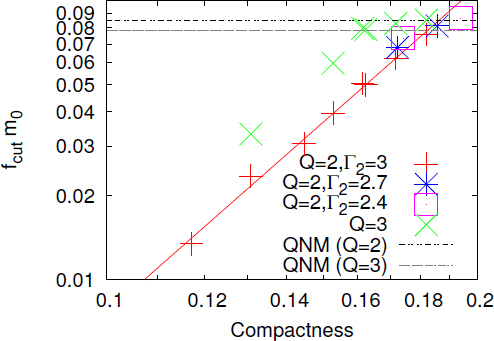
Gc−3fcut
m0 as a function of  in logarithmic scales. The solid line is obtained by a linear fitting of the data for Q = 2 and Γ2 = 3. The short-dashed and long-dashed lines show approximate frequencies of the QNM of the remnant BH for Q = 2 and Q = 3, respectively. This figure is taken from [107].
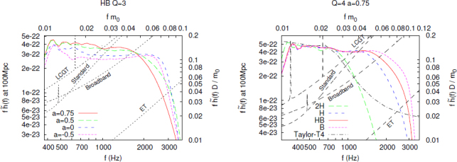
Left: The same as Figure 26 but for Q = 3, MNS = 1.35 M⊙, and a = 0.75, 0.5, 0, and −0.5 with a moderately stiff EOS (EOS HB). Right: The same as the left panel but for Q = 4, a = 0.75, and MNS = 1.35 M⊙ with various EOS. The thin dashed curves show the noise curves for LCGT, advanced LIGO, broadband-designed advanced LIGO, and Einstein telescope (from upper to lower). The figures are taken from [109].
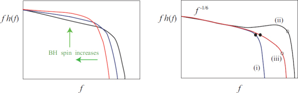
Left: Schematic figure of the type-I gravitational-wave spectrum for a high-frequency side with different values of the BH spin but for the same masses of BH and NS, and NS EOS. With increase of the BH spin, the cutoff frequency decreases and the amplitude below the cutoff frequency increases. Right: Three types of the gravitational-wave spectrum. Type-I (i) and type-II (ii) are the same as those shown in Figure 27. Type-III (iii) is shown for the case in which the BH spin is high and the mass ratio (and thus the area of the BH horizon) is large. The filled and open circles denote the cutoff frequencies associated with tidal disruption and with a QNM, respectively.
References
-
- Abadie J, LIGO Scientific Collaboration et al. Calibration of the LIGO Gravitational Wave Detectors in the Fifth Science Run. Nucl. Instrum. Methods A. 2010;624:223–240. doi: 10.1016/j.nima.2010.07.089. - DOI
-
- Abbott BP, LIGO Scientific Collaboration et al. LIGO: the Laser Interferometer Gravitational-Wave Observatory. Rep. Prog. Phys. 2009;72:076901. doi: 10.1088/0034-4885/72/7/076901. - DOI
-
- Accadia T, Virgo Collaboration et al. Calibration and sensitivity of the Virgo dector during its second science run. Class. Quantum Grav. 2011;28:025005. doi: 10.1088/0264-9381/28/2/025005. - DOI
-
- Acernese F, Virgo Collaboration et al. Status of VIRGO. Class. Quantum Grav. 2008;25:114045. doi: 10.1088/0264-9381/25/11/114045. - DOI
-
- Ajith P, et al. Template bank for gravitational waveforms from coalescing binary black holes: Nonspinning binaries. Phys. Rev. D. 2008;77:104017. doi: 10.1103/PhysRevD.77.104017. - DOI
Publication types
LinkOut - more resources
Full Text Sources
Miscellaneous