Measurements and models of electric fields in the in vivo human brain during transcranial electric stimulation

Abstract

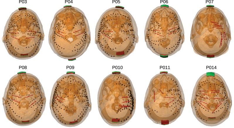
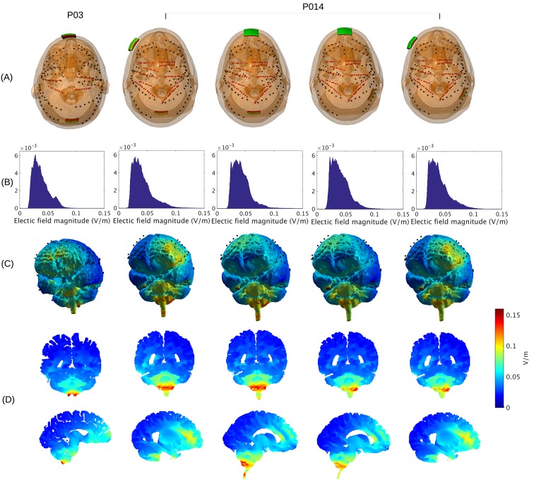
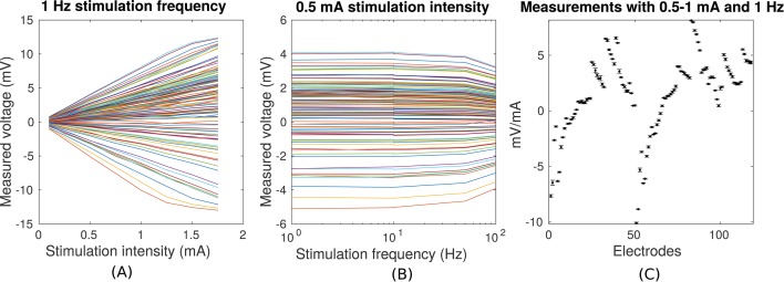
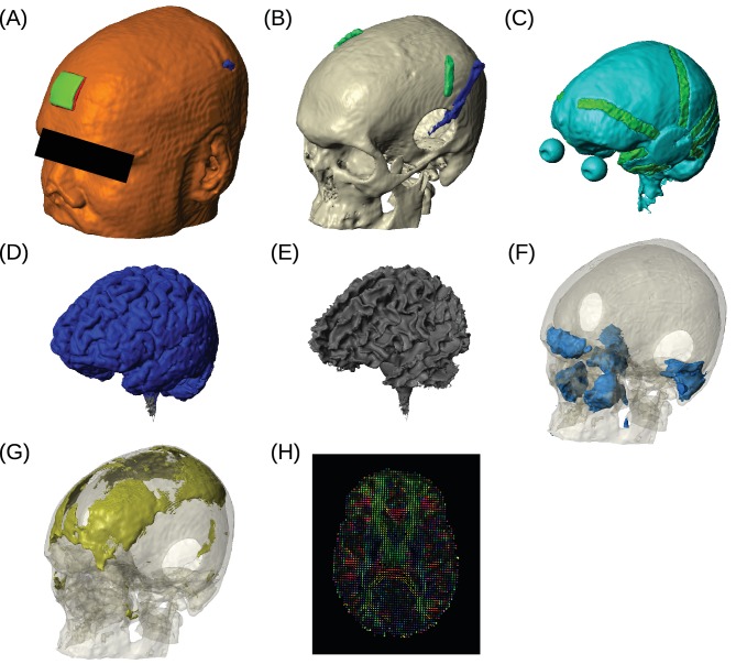
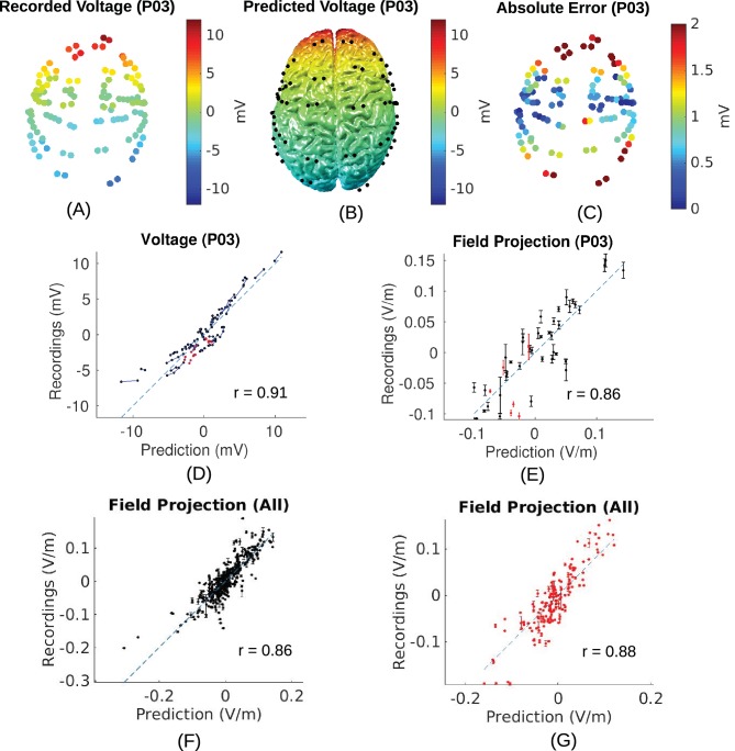
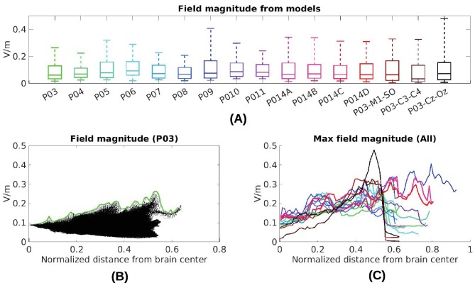
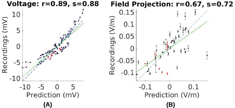
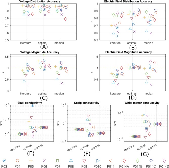
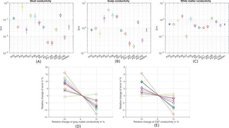
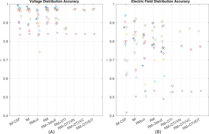
Transcranial electric stimulation aims to stimulate the brain by applying weak electrical currents at the scalp. However, the magnitude and spatial distribution of electric fields in the human brain are unknown. We measured electric potentials intracranially in ten epilepsy patients and estimated electric fields across the entire brain by leveraging calibrated current-flow models. When stimulating at 2 mA, cortical electric fields reach 0.8 V/m, the lower limit of effectiveness in animal studies. When individual whole-head anatomy is considered, the predicted electric field magnitudes correlate with the recorded values in cortical (r = 0.86) and depth (r = 0.88) electrodes. Accurate models require adjustment of tissue conductivity values reported in the literature, but accuracy is not improved when incorporating white matter anisotropy or different skull compartments. This is the first study to validate and calibrate current-flow models with in vivo intracranial recordings in humans, providing a solid foundation to target stimulation and interpret clinical trials.

Keywords: computational current-flow model; human; intracranial recordings; neuroscience; transcranial electric stimulation.

Figure 1.. Location of the invasive recording electrodes and transcranial electrical stimulation electrodes in the 10 patients tested.

Electrodes measuring from the cortical surface (64-contact grids, 8-contact strips) are indicated as black dots and depth electrodes (between 6–8 contacts each) as red dots. Square stimulation electrodes on scalp surface (2 cm), are shown in green with contact gel in red. Individual anatomy derived from the T1-weighted MRI is transparent to visualize electrode locations. DOI: http://dx.doi.org/10.7554/eLife.18834.002

Figure 2.. Prediction of electric field with calibrated models for various electrode montages at 1 mA stimulation intensity.

(B) Histogram of electric field magnitude for the montage used on Subject P03 (same as in Figure 5) and Subject P014. (C) Corresponding spatial distributions on cortical surface. (D) Cross-section plots showing predicted electric field intensity in mid-brain areas with hot spots underneath stimulation electrodes and adjacent to highly conducting ventricles. DOI: http://dx.doi.org/10.7554/eLife.18834.003

Figure 3.. Voltage recordings across multiple intracranial locations for sinusoidal transcranial alternating current stimulation for the first subject tested (P03).

Magnitude and sign are estimated by fitting a sinusoid to the voltage fluctuations at each electrode location. (A) Voltage recordings at multiple intracranial recording locations are linear with stimulation intensity up to 1 mA in this subject (each curve represents a different electrode). At higher intensities some channels saturate due to a limited dynamic range of the clinical recording equipment, which is demonstrated by the plateauing of measured voltage at intensities above 1.5 mA. (B) Intensities are constant with frequency in the range of 1–10 Hz. The drop-off at higher frequencies is due to the recording equipment. (C) Averaged measurements across three stimulation sessions (separated by approximately 1 min each) demonstrate stability of electric field measurements across sessions. (Here stimulation was 1 Hz and between 0.5–1 mA in stimulation current. The voltage values are calibrated to correspond to 1 mA stimulation). Error bars at each electrode indicate the variability across different stimulation blocks. DOI: http://dx.doi.org/10.7554/eLife.18834.004

Figure 4.. Example of realistic model for Subject P06.

Each patient's detailed anatomy was obtained by segmenting T1-weighted MR images into six tissue types: scalp, skull, CSF, gray matter, white matter, and air. Additionally, to capture the surgical details we modeled the craniotomy, cortical strips and depth electrodes as well as the subgaleal electrodes. Finite element models were built and solved to compute voltages and electric fields throughout the head. (A) Scalp, with stimulating pad electrode; configuration used here is the same as shown in Figure 1. (B) Skull, note the Jackson-Pratt Drain (blue), the subgaleal electrodes (green) and the craniotomy. (C) CSF, with the geometry of intracranial electrode strips. Craniotomy site was assumed to be filled with CSF. (D) Gray matter. (E) White matter. (F) Air cavities. (G) Spongy bone inside the skull. (H) Diffusion tensor distribution in one brain slice. DOI: http://dx.doi.org/10.7554/eLife.18834.005

Figure 5.. Voltage and electric field for measurements and model.

All values are calibrated to 1 mA stimulation. (A) False-color representation of measured voltages for patient P03. (B) Voltages from the corresponding individualized model across the cortical surface. (C) Absolute voltage difference between recording and model predictions. (D) Comparison of recorded voltages with values predicted by the individualized model for P03. Each point in the scatter plot represents an intracranial electrode as shown in (A), with black indicating cortical surface electrodes and red representing depth electrodes (mostly targeting hippocampus). (E) Projected electric field is measured in the direction of nearby electrodes (pairs connected by blue lines in (D)), and is calculated as the voltage difference divided by the distance between the two electrodes. Error bar at each point indicates the standard variation of the measured electric field at the corresponding electrode as shown in Figure 3C). (F) Projected electric field for cortical surface recordings and corresponding model predictions combining all the subjects. (G) Same as (F) showing all the depth electrodes. DOI: http://dx.doi.org/10.7554/eLife.18834.006

Figure 6.. Electric field predicted with individually calibrated models under 1 mA stimulation.

(A) Summary of electric field magnitudes for all subjects. The four different configurations of stimulation electrodes in Subject P014 are indicated as P014A–P014D. Also shown are values for a few stimulation montages commonly used in clinical trials simulated for Subject P03 (M1–SO, C3–C4, Cz–Oz). Whiskers indicate the maximal and minimal values of electric field magnitudes observed across the entire brain, and box indicates the 5% and 95% percentile across locations. Line inside the box indicates median value. (B) Electric field magnitudes as a function of depth, measured as the distance from the origin of the MNI coordinate system and normalized by diameter of the brain. Maximal field value is achieved at the cortical surface, which is approximately at distance of 0.55 (distance was divided by brain diameter in each MNI dimension). Locations exceeding 0.55 indicate mostly brain stem and cerebellum. Maximal value for each depth is indicated in green. (C) Summary of maximum for each of the 10 subjects and montages shown in (A) as a function of depth. DOI: http://dx.doi.org/10.7554/eLife.18834.008

Figure 7.. Comparison of recorded values with model predictions using literature conductivity values for Subject P03 scaled to 1 mA.

Points falling on the dashed blue line represent perfect prediction (slope s = 1). The literature values gives close estimates of electric field magnitude (measurements are 72% of predicted values, s = 0.72, green line). Skin, skull and brain conductivities are optimized to minimize prediction error for field projections (i.e. minimize mean square distance from dashed line in panel (B)) which corrects this magnitude mismatch, and is shown in Figure 5E. DOI: http://dx.doi.org/10.7554/eLife.18834.009

Figure 8.. Prediction accuracy for models using various conductivity choices.

(A, B) Correlation indicates the accuracy of the spatial distribution. (C, D) Slope indicates the accuracy of the magnitude estimate. Results are shown for three categories of models: models using literature conductivities (literature), models using individually optimized conductivities for skull, scalp and brain to provide best fit to the measured electric fields in each subject (optimal), and models with the median of the optimal conductivities (median of P03–P011 and P014). Each subject is represented by a different symbol as indicated by the legend on the bottom of the figure. P014A–P014D represent the four different configurations of stimulation electrodes in P014. Panels (E) – (G) summarize different optimal conductivities for different individuals. DOI: http://dx.doi.org/10.7554/eLife.18834.010

Figure 8—figure supplement 1.. Estimation of the sensitivity of the fitting procedure to small variations in the conductivity values.

(A–C) For conductivities that were fit to the data (skull, scalp, white matter) we numerically evaluated the Cramér-Rao bound, shown here as error bars around the optimal values for each subject, and the median values. (D–E) For conductivities that were held constant (gray matter and CSF) we varied here the values by 10% and report the relative change of the fitting criterion (Equation 1) as % change. DOI: http://dx.doi.org/10.7554/eLife.18834.011

Figure 9.. Performance of various modeling approaches.

IM-CSF: This ‘intact model’ is based on the pre-surgical MRI and does not include craniotomy, recording electrodes, etc., and does not model CSF either; IM: intact model including CSF; RMcut: realistic model with all details as shown in Figure 4A–F, but truncated at the bottom of the skull due to the limited FOV of the clinical MRI scans; RM: realistic model with an extended FOV including the lower head and neck based on a standard head model; RM + 3skull: realistic model including 3-compartment skull as shown in Figure 4G; RM+DTI: realistic model including DTI as shown in Figure 4H. Four different ways to convert DTI ellipsoids into estimated anisotropic conductivity values were tested: direct method (DTI), volume normalized (DTI/VN), volume constrained (DTI/VC), and equivalent isotropic trace (DTI/EIT). What is demonstrated is that truncated head models may deteriorate prediction accuracy, and models accounting for CSF, multiple skull compartments or white matter tracts do not significantly improve model accuracy. DOI: http://dx.doi.org/10.7554/eLife.18834.012

References

1. Acar ZA, Makeig S. Neuroelectromagnetic forward head modeling toolbox. Journal of Neuroscience Methods. 2010;190:258–270. doi: 10.1016/j.jneumeth.2010.04.031. - DOI - PMC - PubMed
1. Akhtari M, Bryant HC, Mamelak AN, Flynn ER, Heller L, Shih JJ, Mandelkern M, Matlachov A, Ranken DM, Best ED, DiMauro MA, Lee RR, Sutherling WW. Conductivities of three-layer live human skull. Brain Topography. 2002;14:151–167. doi: 10.1023/A:1014590923185. - DOI - PubMed
1. Alam M, Truong DQ, Khadka N, Bikson M. Spatial and polarity precision of concentric high-definition transcranial direct current stimulation (HD-tDCS) Physics in Medicine and Biology. 2016;61:4506–4521. doi: 10.1088/0031-9155/61/12/4506. - DOI - PubMed
1. Alekseichuk I, Diers K, Paulus W, Antal A. Transcranial electrical stimulation of the occipital cortex during visual perception modifies the magnitude of BOLD activity: a combined tES-fMRI approach. NeuroImage. 2016;140 doi: 10.1016/j.neuroimage.2015.11.034. - DOI - PubMed
1. Ali MM, Sellers KK, Fröhlich F. Transcranial alternating current stimulation modulates large-scale cortical network activity by network resonance. Journal of Neuroscience. 2013;33:11262–11275. doi: 10.1523/JNEUROSCI.5867-12.2013. - DOI - PMC - PubMed
Publication types